This post has been republished via RSS; it originally appeared at: Excel Blog articles.
We are excited to announce that it is now possible to insert new Pivot Tables in Excel Online.
This was one of the top requests from our community and we have now rolled it out for all of our Office Online customers.
To learn more about Pivot Tables please use this overview article and our new Pivot Table Tutorial.
Before you get started
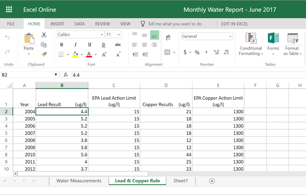
- Your data should be organized in a tabular format. Ideally, you can use an Excel table (select the grid data and use Format as Table in the HOME tab). Tables are a great source of data for Pivot Tables because rows added to the “source” Table (later on) will be automatically included in the Pivot Table once you refresh it.
- Data types in columns should be the same. For example, you shouldn't mix dates and text in the same column. Also, you’ll get the best results if the “source” data doesn’t have any blank rows or columns.
Select the “source” data you want to analyze
Just stand on the data. You don’t even have to select it all. If you do select a region, your selection will be respected.
Insert Pivot Table
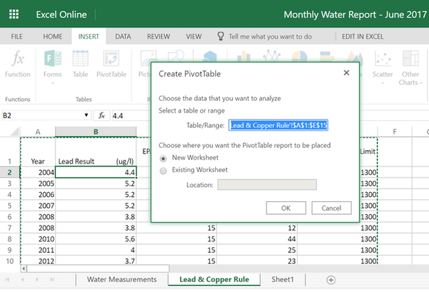
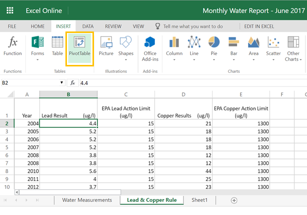
Go to INSERT tab and press PivotTable:
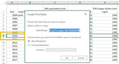
The Create PivotTable dialog will open, and unless you selected a region, the whole Table/Range will automatically be selected as the data you want to analyze:
At this point, you can just click OK, and the new Pivot Table will get added to a new worksheet, just like in Excel Desktop application.
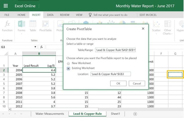
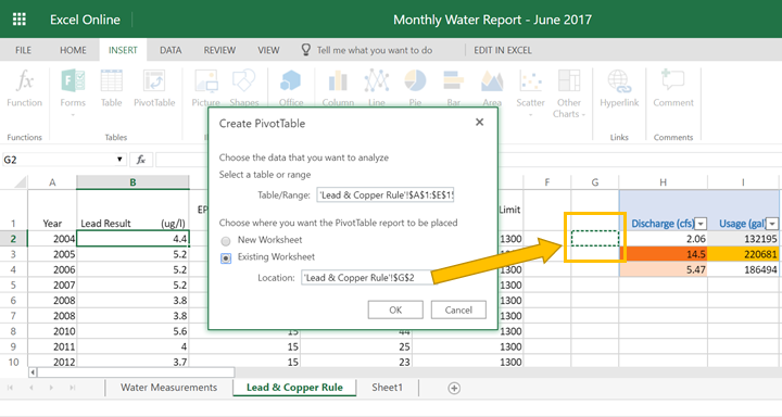
You also have the option to select an alternative location - press Existing Worksheet and then click the desired location:
Inserted it. Now what?
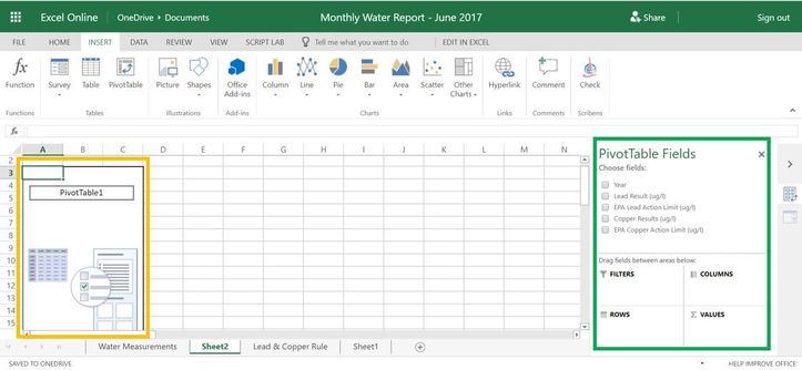
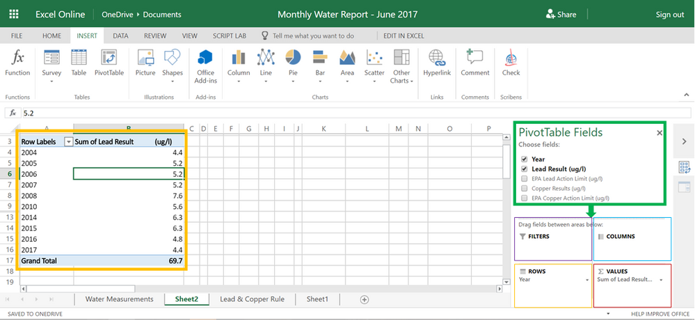
Once you insert a Pivot Table, you will see something like this on your screen:
As enigmatic as it might look, this actually means you are all set to go and do your analysis!
The yellow outline (above) is the placeholder for your new Pivot Table – that’s where you’ll see your newly formed Pivot Table, once you define it.
The green outline (above) is where you define how your new Pivot Table will look like.
To define the look of your new Pivot Table, all you need to do is drag PivotTable Fields into the four areas, as outlined below. And if you want to remove some field you dragged in, just drag it out and drop – it’ll go away.
Pitfalls & Limitations
Excel Online doesn’t support some of the less common capabilities of Excel desktop application, as outlined below:
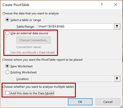
All other constraints of the feature are the same as in Excel desktop application.
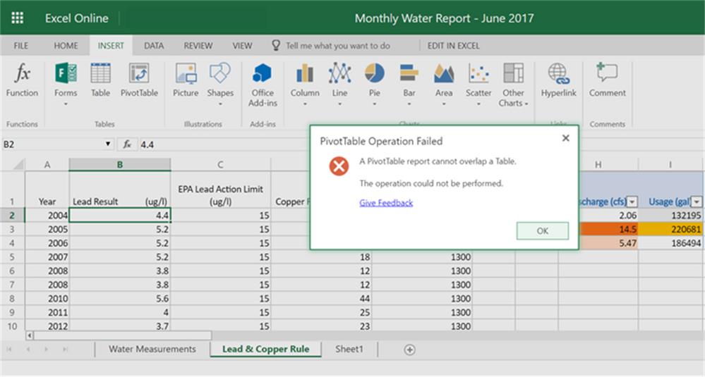
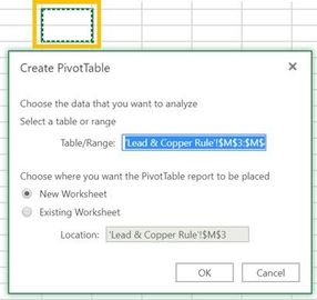
For example, you cannot add a pivot table to a location that is too close to an existing table:
If you try to do that, you’ll get the following error message:
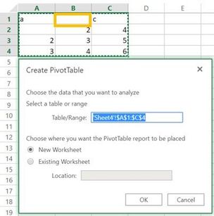
Another common pitfall is to try and use a piece of data that isn’t suitable for pivoting.
If you try to create a Pivot Table on top of such invalid “source” data, you’ll get an error.
The “source” data is considered invalid in either one of these cases:
● Your “source” data points to an empty range (so, there is nothing to pivot)
● Your “source” data has a column without a header (so, there is no way to relate to it in a PivotTable)
● Your “source” data points to a single row (so, there is nothing to pivot)

