This post has been republished via RSS; it originally appeared at: New blog articles in Microsoft Tech Community.
This past semester we have been collaborating on a machine learning Capstone Project with Columbia University’s Master of Science in Applied Analytics: capstone projects are applied and experimental projects where students take what they have learned throughout the course of their graduate program and apply it to examine a specific area of study.
Capstone projects are specifically designed to encourage students to think critically, solve challenging data science problems, and develop analytical skills. Two group of students built an end-to-end data science solution using Azure Machine Learning to accurately forecast sales. Azure Machine Learning is a cloud-based environment that you can use to train, deploy, automate, manage, and track ML models.
Azure Machine Learning can be used for any kind of machine learning, from classical machine learning to deep learning, supervised, and unsupervised learning. Whether you prefer to write Python or R code or zero-code/low-code options such as the designer, you can build, train, and track highly accurate machine learning and deep-learning models in an Azure Machine Learning Workspace.
To explore the solution developed by students at Columbia University, you can look at their Time-Series-Prediction repository on GitHub. In this article, we use an approach also used by Columbia University students, which is Automated Machine Learning (Automated ML or AutoML) to train, select, and operationalize a time-series forecasting model for multiple time-series. Make sure you have executed the configuration notebook before running this notebook.
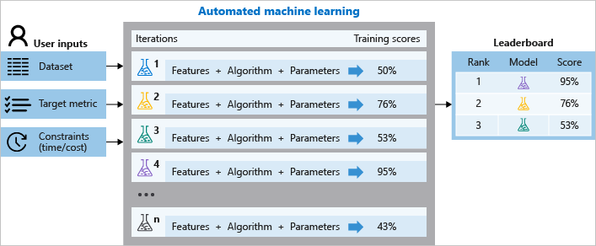
Automated ML (as illustrated in Figure 1 below) is the process of automating the time consuming, iterative tasks of machine learning model development. It allows data scientists, analysts, and developers to build ML models with high scale, efficiency, and productivity all while sustaining model quality:
Figure 1 - Automated ML process on Azure - Source: www.aka.ms/AutomatedMLDocs
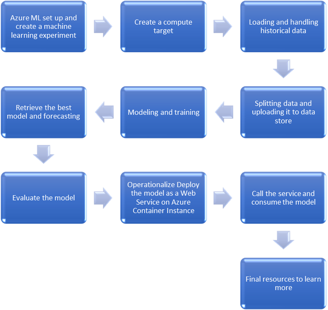
The examples below use the Dominick's Finer Foods data set from James M. Kilts Center, University of Chicago Booth School of Business, to forecast orange juice sales. In the rest of this article we will go through the following steps:
1. Azure ML set up and create a machine learning experiment
As part of the setup you have already created a Workspace. To run AutoML, you also need to create an Experiment. An Experiment corresponds to a prediction problem you are trying to solve, while a Run corresponds to a specific approach to the problem:
2. Create a compute target
You will need to create a compute target for your AutoML run. In this tutorial, you create AmlCompute as your training compute resource.
If the AmlCompute with that name is already in your workspace this code will skip the creation process. As with other Azure services, there are limits on certain resources (e.g. AmlCompute) associated with the Azure Machine Learning service:
3. Loading and handling historical data
You are now ready to load the historical orange juice sales data. We will load the CSV file into a plain pandas DataFrame; the time column in the CSV is called WeekStarting, so it will be specially parsed into the datetime type:
Each row in the DataFrame holds a quantity of weekly sales for an OJ brand at a single store. The data also includes the sales price, a flag indicating if the OJ brand was advertised in the store that week, and some customer demographic information based on the store location. For historical reasons, the data also include the logarithm of the sales quantity. The Dominick's grocery data is commonly used to illustrate econometric modeling techniques where logarithms of quantities are generally preferred.
The task is now to build a time-series model for the Quantity column. It is important to note that this dataset is comprised of many individual time-series - one for each unique combination of Store and Brand. To distinguish the individual time-series, we thus define the grain - the columns whose values determine the boundaries between time-series:
For demonstration purposes, we extract sales time-series for just a few of the stores:
4. Splitting data and uploading it to data store
We now split the data into a training and a testing set for later forecast evaluation. The test set will contain the final 20 weeks of observed sales for each time-series. The splits should be stratified by series, so we use a group-by statement on the grain columns:
The Machine Learning service workspace, is paired with the storage account, which contains the default data store. We will use it to upload the train and test data and create tabular datasets for training and testing:
5. Modeling and training
For forecasting tasks, AutoML uses pre-processing and estimation steps that are specific to time-series. Automated ML will undertake the following pre-processing steps:
- Detect time-series sample frequency (e.g. hourly, daily, weekly) and create new records for absent time points to make the series regular. A regular time series has a well-defined frequency and has a value at every sample point in a contiguous time span
- Impute missing values in the target (via forward-fill) and feature columns (using median column values)
- Create grain-based features to enable fixed effects across different series
- Create time-based features to assist in learning seasonal patterns
- Encode categorical variables to numeric quantities
In this notebook, AutoML will train a single, regression-type model across all time-series in a given training set. This allows the model to generalize across related series. If you're looking for training multiple models for different time-series, please check out the forecasting grouping notebook.
You are almost ready to start an AutoML training job. First, we need to separate the target column from the rest of the DataFrame:
The AutoMLConfig object defines the settings and data for an AutoML training job. Here, we set necessary inputs like the task type, the number of AutoML iterations to try, the training data, and cross-validation parameters.
For forecasting tasks, there are some additional parameters that can be set: the name of the column holding the date/time, the grain column names, and the maximum forecast horizon. A time column is required for forecasting, while the grain is optional. If a grain is not given, AutoML assumes that the whole data set is a single time-series. We also pass a list of columns to drop prior to modeling.
The logQuantity column is completely correlated with the target quantity, so it must be removed to prevent a target leak.
The forecast horizon is given in units of the time-series frequency; for instance, the OJ series frequency is weekly, so a horizon of 20 means that a trained model will estimate sales up to 20 weeks beyond the latest date in the training data for each series. In this example, we set the maximum horizon to the number of samples per series in the test set (n_test_periods). Generally, the value of this parameter will be dictated by business needs. For example, a demand planning organization that needs to estimate the next month of sales would set the horizon accordingly.
Finally, a note about the cross-validation (CV) procedure for time-series data. AutoML uses out-of-sample error estimates to select a best pipeline/model, so it is important that the CV fold splitting is done correctly. Time-series can violate the basic statistical assumptions of the canonical K-Fold CV strategy, so AutoML implements a specific procedure to create CV folds for time-series data. To use this procedure, you just need to specify the desired number of CV folds in the AutoMLConfig object. It is also possible to bypass CV and use your own validation set by setting the validation_data parameter of AutoMLConfig:
You can now submit a new training run. Depending on the data and number of iterations this operation may take several minutes. Information from each iteration will be printed to the console:
6. Retrieve the best model and forecasting
Each run within an Experiment stores serialized (i.e. pickled) pipelines from the AutoML iterations. We can now retrieve the pipeline with the best performance on the validation data set:
Now that we have retrieved the best pipeline/model, it can be used to make predictions on test data. First, we remove the target values from the test set:
To produce predictions on the test set, we need to know the feature values at all dates in the test set. This requirement is somewhat reasonable for the OJ sales data since the features mainly consist of price, which is usually set in advance, and customer demographics which are approximately constant for each store over the 20 week forecast horizon in the testing data:
If you are used to scikit pipelines, perhaps you expected predict(X_test). However, forecasting requires a more general interface that also supplies the past target y values. Please use forecast(X,y) as predict(X) is reserved for internal purposes on forecasting models.
7. Evaluate the model
To evaluate the accuracy of the forecast, we'll compare against the actual sales quantities for some select metrics, included the mean absolute percentage error (MAPE).
It is a good practice to always align the output explicitly to the input, as the count and order of the rows may have changed during transformations that span multiple rows:
8. Operationalization: deploy the model as a Web Service on Azure Container Instance
Operationalization means getting the model into the cloud so that other can run it after you close the notebook. We will create a docker running on Azure Container Instances with the model:
For the deployment we need a function which will run the forecast on serialized data. It can be obtained from the best_run:
9. Call the service and consume the model
Finally, in order to call the service and consume your machine learning model, you can run the following script:
10. Final resources to learn more
To learn more, you can read the following articles and notebooks:
- Azure Machine Learning Notebooks: aka.ms/AzureMLServiceGithub
- Azure Machine Learning Service: aka.ms/AzureMLservice
- Get started with Azure ML: aka.ms/GetStartedAzureML
- Automated Machine Learning Documentation: https://aka.ms/AutomatedMLDocs
- What is Automated Machine Learning? https://aka.ms/AutomatedML
- Model Interpretability with Azure ML Service: https://aka.ms/AzureMLModelInterpretability
- Azure Notebooks: https://aka.ms/AzureNB
- Python Microsoft: https://aka.ms/PythonMS
- Azure ML for VS Code: aka.ms/AzureMLforVSCode


