This post has been republished via RSS; it originally appeared at: Microsoft Research.
Reinforcement Learning (RL), much like scaling a 3,000-foot rock face, is about learning to make sequential decisions. The list of potential RL applications is expansive, spanning robotics (drone control), dialogue systems (personal assistants, automated call centers), the game industry (non-player characters, computer AI), treatment design (pharmaceutical tests, crop management), complex systems control (for resource allocation, flow optimization), and so on.
Some RL achievements are quite compelling. For example, Stanford University’s RL team learned how to control a reduced model helicopter, and even learned new aerobatics with it. Orange Labs deployed the first commercial dialogue system optimized with RL. DeepMind invented DQN, the first deep RL algorithm capable of playing Atari games at human skill level using visual inputs, and were able to train a Go AI by playing it solely against itself. It reigns undefeated in its Go matches against human players.
Despite such remarkable achievements, applying RL to most real-world scenarios remains a challenge. There are several reasons for this. Deep RL algorithms are not sample efficient; they require billions of samples to obtain their results and extracting such astronomical numbers of samples in real world applications isn’t feasible. RL also falls short in the area of morality constraints; the algorithms need to be safe. They have to be able to learn in real-life scenarios without risking lives or equipment. The RL algorithms also need to be fair; they must ensure they are not discriminating against people. Finally, the algorithms need to be reliable and deliver consistently solid results.
This blog post focuses on reliability in reinforcement learning. Deep RL algorithms are impressive, but only when they work. In reality, they are largely unreliable. Even worse, two runs with different random seeds can yield very different results because of the stochasticity in the reinforcement learning process. We propose two ways of mitigating this.
Algorithm Selection
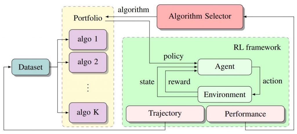
The first idea (published last year at ICLR) is quite simple. If one algorithm is not reliable, we train several of them and use the best one. Figure 1 illustrates the algorithmic selection process. At the beginning of each episode, the algorithm selector selects an algorithm from the Portfolio. The selected algorithm outputs a policy that will be utilized for the entirety of the subsequent episode. Then, in the green area, the standard RL loop runs until the completion of the episode. The generated trajectory is recorded and fed to the algorithms for future training. The performance measure is sent to the algorithm selector, so that it selects the fittest algorithms in the future.
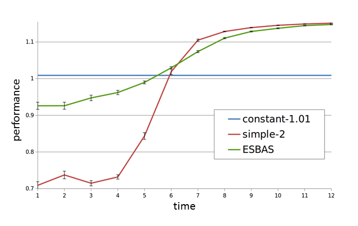
Preliminary experiments in this study were conducted using a negotiation dialogue game. Focusing on one particular portfolio, our system, denoted by ESBAS, was composed of only two algorithms. The performance of each algorithm over time is displayed on Figure 2. The first algorithm, in blue, constantly generates the same policy with performance 1, while the second one, in red, learns over time. ESBAS, in green, hands in a performance approaching that of the best algorithm at each time step. Indeed, overall ESBAS enjoys a better performance than either of the other two. We pursued the empirical validation on an Atari game called Q*bert. Making several DQN architectures compete, we found out that our system yielded a better final performance than any single architecture on its own.
We’d previously argued ESBAS improves the reliability of the RL algorithms, but in fact it has other virtues. First; it allows staggered learning, preferentially using the algorithm with the best policy at each time step. Second, it allows the use of objective function that may not be directly implemented as rewards (for instance it allows enforcement of safety constraints.) Third, we observe that the ensemble of policies generated more diverse experience about the environment (and richer diversity usually results in richer information). And finally, as we’ve observed with the constant algorithm, EBAS allows smooth transfer between a baseline policy and a learned policy.
Reliable Policy Improvement
Our second stab at improving the reliability of RL algorithms focused on one specific setting, often encountered in real world applications: batch reinforcement learning. Compared to the classical online setting, in batch reinforcement learning the learning agent does not interact directly with the environment (see Figure 3.). Instead, it is a baseline agent. It is fixed and is used to collect data that then is fed into an algorithm to train a new policy. The batch setting is a constraint commonly encountered in real world scenarios. Dialogue systems or video games generally are deployed on personal devices, making it difficult to update frequently. In other settings, such as pharmaceutical tests or crop management, the time scale is so long – we’re talking several years – that you need to run the trajectories in parallel, therefore requiring using the same policy.
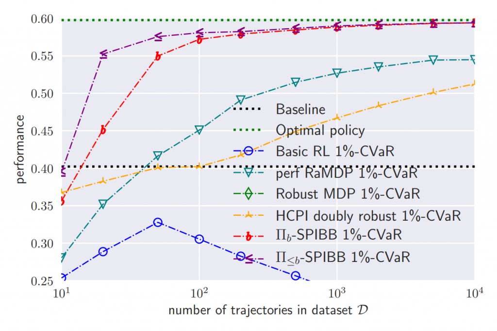
Classic RL algorithms improve on average the baseline. Unfortunately, they cannot do so reliably. Reliable policy improvement is crucial in batch settings because if a policy is bad, it will remain bad for many trajectories. We want algorithms to almost always improve the baseline policy. In order to look at the worst-case scenarios, we looked at the Conditional value at Risk (CvaR). CvaR is actually a simple concept; it is the average of the worst runs. Here, a run is defined as the batch process shown on Figure 3 (data collection and policy training). 1%-CVaR therefore signifies the average of performance over the 1% worst runs.
It is important to explain why classic RL fails. Its only source of information is the dataset that classic RL algorithms implicitly or explicitly use as the proxy for the true environment. But, because of the environment stochasticity or the model function approximation, the proxy is uncertain when the evidence is limited by the dataset. Consequently, the learning algorithm that only has the dataset for information, has many blind spots, and may be over-reliant on the dataset. As a result, classic RL occasionally trains policies that are very bad in the true environment.
And indeed, it’s actually worse than that; reinforcement learning will search and find a way to optimize the objective function. It has been shown to be effective at finding and exploiting glitches in games–certainly fun in that context. But in a batch setting, you do not want your algorithm to exploit glitches, because the glitches are likely to be fantasized from the blind spots in your data. And the more complex the domain is, the more blind spots you get. Therefore, it’s imperative to ensure that the algorithm is careful with the blind spots.
We solved this challenge by designing a new algorithm called SPIBB (Safe Policy Improvement with Baseline Bootstrapping), in work to be presented at the 2019 International Conference on Machine Learning (ICML 2019). SPIBB implements the following commonsensical rule to the policy update: if you don’t know what you’re doing, don’t do it. More precisely, if there is sufficient data to support the policy change, then it is allowed to do so. Otherwise, just reproduce the baseline policy that was used during the data collection. Soft-SPIBB (presented at EWRL 2018) is a variant of the same idea with a softer rule: the policy change is allowed to be changed up to the inverse to the measured uncertainty. SPIBB has also been adapted to factored MDPs (one presented at AAAI 2019 and another to be presented at IJCAI 2019).
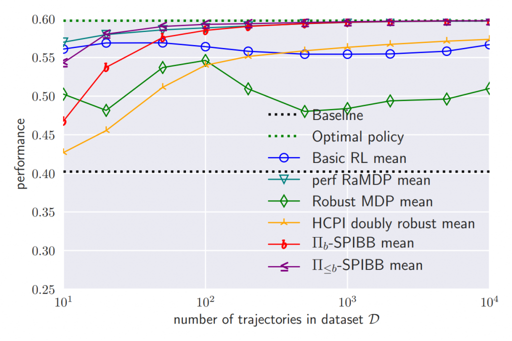
We performed a benchmark on a stochastic gridworld environment with only 25 states and four actions. Depending on the size of the dataset, displayed on the x-axis on a log-scale, we observed the average performance of several algorithms in the literature (see Figure 4.) The baseline performance is shown as a black dotted line in the middle of the figure. All the algorithms improve upon it, on average. We display two variants of the SPIBB algorithm, in red and in purple. Both are among the best algorithms in mean score. In particular, we observe that the classic RL, shown in blue, surprisingly does not really improve with the size of the dataset. The only algorithm on-par or even arguably better than SPIBB is RaMDP, in light blue, which has two shortcomings: it relies on a hyperparameter that needs to be very finely tuned and it is not as reliable as the SPIBB algorithms.
Figure 5 showed the mean performance, but we are more interested in the reliability of the trained policies. We measure the 1%-CVaR and display it on Figure 5. We observe that basic reinforcement learning (blue), is unreliable. The most reliable algorithms are versions of SPIBB, by a wide margin. As mentioned earlier, RaMDP is unreliable with small datasets.
Similar results have been obtained on small random environments, with random baselines. The study also provides formal proofs of the reliability of SPIBB in finite MDPs. Finally, the study demonstrated SPIBB efficiency and reliability on a larger continuous navigation task, using deep reinforcement learning with even better results in comparison with the other algorithms. A larger set of results will further be presented at RLDM 2019.
I look forward to demonstrating these ideas and getting input at ICML 2019 later this month. In the meantime, be secure, use a good reliable snap hook to work your way up to the pinnacle of deep RL practice and do feel welcome to share your pictures!
The post Reliability in Reinforcement Learning appeared first on Microsoft Research.


