This post has been republished via RSS; it originally appeared at: Excel Blog articles.
For many, it’s that time of year again when budgets need to be dusted down and re-vamped. Those in finance spend sleepless nights reviewing minutiae and “normalizing” data before talking to their operational counterparts.
Sound familiar? Well, Excel can help.
What I want to talk about is the need for objective forecasting. By this, I mean something that can be constructed simply such that if anyone follows the same process, they will get the same figures. This needs to be a mechanical, objective process. This way, analysts may prepare this data in moments. Operational managers can review the trend and state and all they need to do is explain the variation, i.e. undertake incremental budgeting. Both parties should work together as a team.
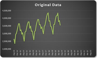
What we need is a process. As an example, consider the following:
The aim is to develop a technique to identify what would be next in a series, i.e. forecast the future. There are various approaches you could use: simple average, moving average, weighted moving average, etc.
All these approaches are simplistic and have obvious flaws. A slightly more sophisticated method is called regression analysis: well, that takes me back! This is a technique where you plot an independent variable on the x (horizontal axis) against a dependent variable on the y (vertical) axis. “Independent” means a variable you may select (e.g. “June”, “Product A”) and dependent means the result of that choice or selection.
Let’s return to my example:
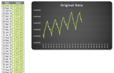
Now let’s be honest, anyone who has historical data looking this perfect should be referred to the auditors, but hey, this is for illustration purposes. I have data from August 2014 until last month. I want to extrapolate it beyond 2020 (I want 2020 foresight!).
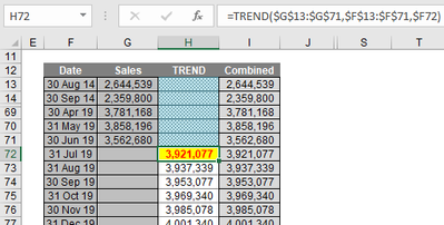
There are several functions that can help us here, with one of the simplest being TREND. TREND(known_y’s,known_x’s,new_x’s,[constant]) projects assuming that there is a relationship between two sets of variables x (independent variable – here, the dates) and y (dependent variable – the sales).
It’s preferable to leave constant blank in the TREND function in order to obtain the best fit. For example:
Hence, we can extrapolate the data using the TREND function.
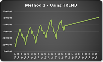
Ladies and gentleman, you may have heard of hockeystick projections; well, let me now present you with the swordfish. You extrapolate linearly, you get a straight line. Well duh.
This isn’t good enough. We need to identify the cyclicality of the data. It appears to go through a cycle once every 12 months. This might not always be the case, but the concept remains the same even if the periodicity is not annual.
I want to calculate a periodic growth rate objectively.
In my example, I am going to compare the sum of the sales over the 12 months ending 30 June 2019 with the forecast sales as calculated using TREND over the 12 months ending 30 June 2020:
It is this percentage I will use to grow the forecasts.
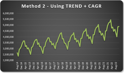
I then grow each period’s value by its corresponding value in the previous period by this percentage (7.83% here). This gives me a more realistic chart:
That looks much better. With practice, this approach doesn’t take that long to prepare. Numbers may be varied from this forecast with the operational manager only having to explain these deviations. It makes life easier all round.
Once the method of assessing inferred growth rates based upon the TREND function have been agreed and what normalisations to historical data should be input, the process becomes much more straightforward. Of course, this method should be used for all forecast inputs separately and not just on their aggregation, otherwise confusion occurs due to sales mix changes, new products, cut-off periods, etc.
But there is an even faster way – if you happen to have Office 365 or Excel 2016 (or later)…
Exponential Triple Smoothing (ETS) sounds like a dairy process, but it actually uses the weighted mean of past values for forecasting. It’s popular in statistics as it adjusts for seasonal variations in data, like in the example above. For those who really need to know, Excel uses a variation of the Holt Winters ETS algorithm. You can read details about this algorithm by doing a quick web search.
In Excel 2016, ETS has gone “native”, i.e. it is a standard feature. This includes both a set of new functions such as FORECAST.ETS and other supporting functions for additional statistics. Your dataset does not need to be perfect, as the functions will accommodate up to 30% missing data.
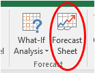
But don’t worry about using these functions. Simply highlight the actual data and click on the ‘Forecast Sheet’ button in the ‘Forecast’ group of the ‘Data’ tab of the Ribbon (ALT + A + FC):
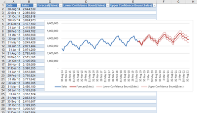
All you need to do is specify the final forecast period at the prompt and that’s it. It produces a raw data sheet, together with confidence intervals (to demonstrate potential spread in the forecast error), which looks something like this:
It’s objective: you select the data and Excel does all the hard yards for you. If you have explained the concept in layman’s terms (as above), then all you need to do is revise the forecast and explain where you wish to change the output from what is generated. Simple!
You may create this longhand. The FORECAST.ETS function calculates or predicts a future value based on existing (historical) values by using this Exponential Triple Smoothing (ETS) algorithm. The predicted value is a continuation of the historical values in the specified target date, which should be a continuation of the timeline. You can use this function to predict future sales, inventory requirements, or consumer trends.
This function requires the timeline to be organised with a constant step between the different points. For example, that could be a monthly timeline with values on the first of every month, a yearly timeline, or a timeline of numerical indices. For this type of timeline, it’s very useful to aggregate raw detailed data before you apply the forecast, which produces more accurate forecast results as well.
The FORECAST.ETS function employs the following syntax to operate:
FORECAST.ETS(target_date, values, timeline, [seasonality], [data_completion], [aggregation])
The FORECAST.ETS function has the following arguments:
- target_date: this is required. This is the data point for which you want to predict a value. The target_date may be date / time or numeric. If the target_date is chronologically before the end of the historical timeline, FORECAST.ETS returns the #NUM!
- values: this is required. The values are the historical values, for which you want to forecast the next
- timeline: this is also required. This is the independent array or range of numeric data. The dates in the timeline must have a consistent step between them and cannot be zero (0). The timeline isn't required to be sorted, as FORECAST.ETS will sort it implicitly for calculations. If a constant step cannot be identified in the provided timeline, FORECAST.ETS will return the #NUM! error. If the timeline contains duplicate values, FORECAST.ETS will return the #VALUE! error. If the ranges of the timeline and values are not of the same size, FORECAST.ETS will return the #N/A
- seasonality: this argument is optional. This is a numeric value with a default value of 1. This means Excel detects seasonality automatically for the forecast and uses positive, whole numbers for the length of the seasonal pattern. 0 indicates no seasonality, meaning the prediction will be linear. Positive whole numbers will indicate to the algorithm to use patterns of this length as the seasonality. For any other value, FORECAST.ETS will return the #NUM!
- The maximum supported seasonality is 8,760 (number of hours in a year). Any seasonality above that number will result in the #NUM!
- data_completion: this argument is also optional. Although the timeline requires a constant step between data points, FORECAST.ETS supports up to 30% missing data, and will automatically adjust for it. Zero (0) will indicate the algorithm to account for missing points as zeros. The default value of 1 will account for missing points by completing them to be the average of the neighboring
- aggregation: this is the final optional argument. Although the timeline requires a constant step between data points, FORECAST.ETS will aggregate multiple points which have the same time stamp. The aggregation parameter is a numeric value indicating which method will be used to aggregate several values with the same time stamp. The default value of 0 will use AVERAGE, while other options are COUNT, COUNTA, MAX, MEDIAN, MIN and SUM.
As for me, I’ll just press the button and keep in mind the simple idea behind it all. After all, during the forecasting season, I’d still like to go home and see the folks.

