This post has been republished via RSS; it originally appeared at: Excel Blog articles.
Have you ever had to repeat the same expression multiple times within a formula, created a mega formula or wished that you had a way to reuse portions of your formula for easier consumption? With the addition of the LET function, now you can!
Introducing LET
LET allows you to associate a calculation or value in your formula with a name. It's names except on a formula level.
The main benefits are:
1. Readability
No more having to remember what a specific range/cell reference referred to, what your calculation was doing or duplicating the same expression within a formula. With the ability to name expressions, you can give meaningful context to readers of your formula.
2. Performance
If you reuse the same expression multiple times in a formula, Excel calculates that expression multiple times. LET allows you to name the expression and refer to it using that name. Any named expression is calculated only once, even if it is referred to many times in the formula. This can significantly improve performance for computationally complex expressions.
The function definition for LET works as follows:
LET(name1, value1, [name2…], [value2…], calculation)
- name1: The name for the 1st value
- value1: The value to associate with the 1st name
- name2 (optional): Additional names
- value2 (optional): Additional values
- calculation: The calculation to perform. This is always the final argument and it can refer to any of the defined names in the LET.
Deconstructing the parameters, there are two things to make note of
1. The names and their values must be in pairs.
For example:
In this case, i) total and ii) SUM(A1:A10) are a pair.
Taking this one step forward, if we wanted to add another name, we just need to define a new pair...
- The last parameter of the function is the calculation which can use the values you named. A properly structured LET will have an odd number of arguments.
In the prior cases this is “total *3” or “total / count”
Example
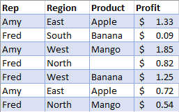
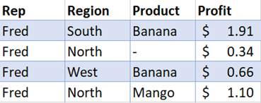
Suppose you have some raw sales data, and you'd like to filter that data to show one person, and add a dash to any blank cells.
| Unfiltered Data | Filtered Data |
 |
 |
This formula can be authored traditionally using the following formula. However, this formula suffers from a common occurrence where you have to make use of the same expression twice, in this case it’s the FILTER expression.
By using a LET we can abstract on this value and even add an addition to fix up the criteria, which in this case is “Fred” but you might want to change to “Amy” in the future or point it at a cell reference.
The other thing to make note of is precedence when referencing names; Name definitions can only make use of prior and not subsequent names. For example, you can see that filterCriteria is able to be used by the filteredRange name definition because it comes afterwards.
An added benefit of using a LET in this formula is that Excel will calculate this formula 2x as fast with the LET because Excel does not have to repeat the same calculation.
Original Formula
|
=IF(ISBLANK(FILTER(A2:D8,A2:A8="Fred")),"-", FILTER(A2:D8,A2:A8="Fred")) |
Formula using LET
|
=LET(filterCriteria, “Fred”, filteredRange, FILTER(A2:D8,A2:A8=filterCriteria), IF(ISBLANK(filteredRange),"-",filteredRange)) |
Learn More
To learn more about LET, please check out our help article.
Availability Notes
LET is now available to Office 365 Subscribers in the Insiders Channel and will be available to users of other channels later this year. I’ll update this blog as LET becomes available to more channels.
In the meantime, please provide feedback either in the comments below or through our normal channels and please note the function signature is subject to change based on feedback before moving to further rings.
To stay connected to Excel and its community, read the Excel blog posts and send us ideas and suggestions via UserVoice. You can also follow Excel on Facebook and Twitter.
Chris Gross
Program Manager, Excel
