This post has been republished via RSS; it originally appeared at: New blog articles in Microsoft Tech Community.
Video Anomaly Detection with Deep Predictive Coding Networks
The code to reproduce this approach can be found on github: https://github.com/Microsoft/MLOps_VideoAnomalyDetection.
Background
The automation of detecting anomalous events in videos is a challenging problem that currently attracts a lot of attention by researchers, but also has broad applications across industry verticals.
One popular approach involves training deep recurrent neural networks to develop an in-depth understanding of the physical and causal rules in the observed scenes, to predict future frames in a video. It is then possible to detect if something unusual occurred in the video, because the model is unable to predict pixel values in the next frame of the video, resulting in a large error in the models prediction.
The approach can be used both in a supervised and unsupervised fashion, thus enabling the detection of predefined anomalies, but also of anomalous events that have never been experienced in the past.
Scenario
To demonstrate how to implement this approach, we will use a publicly available dataset from the University of California, San Diego, which uses stationary cameras to monitor walkways around campus. The goal is to use AI to detect anomalies in the pedestrian traffic on these walkways. Commonly occurring anomalies include bikers, skaters, small carts, and people walking across a walkway or in the grass that surrounds it. The goal is of course not to prosecute the people behind these anomalies, it's just a benchmark dataset for testing this approach.
The approach introduced here is applicable to various other scenarios. In manufacturing, the model can detect accidents on the factory floor (e.g. explosions, disregard of safety guidelines, injuries). In healthcare, it can be used for any kind of visual monitoring (e.g. hallways in hospitals, patients in bed, ultrasound). In financial services, it can be used to detect suspicious behavior (e.g. bank robbery, theft at ATM). In the agricultural industry, it can be used to detect anomalies in the behavior of ranch animals (e.g. limping, predators, thieves). In the education sector, it can be used to detect bullying or other violence in schools or universities.
Outline
In this blog post, I will first provide an overview of the approach. Then I will talk about how to train your model using AML services.
In future blog posts, I will cover these topics:
- Tuning hyperparameters with HyperDrive
- Deploying a real-time webservice for anomaly detection to AKS.
- Defining an AML pipeline that combines all steps from data ingestion and preparation, model training and hyperparameter tuning, model registration, and deployment.
- Performing transfer learning, to quickly scale your solution to new videos.
- Setting up a DevOps build pipeline for retraining your model.
Overview
Neural Network Architecture
Our solution relies an existing architecture (Lotter, W., Kreiman, G. and Cox, D., 2016. Deep predictive coding networks for video prediction and unsupervised learning. arXiv preprint arXiv:1605.08104.). The source code of the original architecture is available on github.
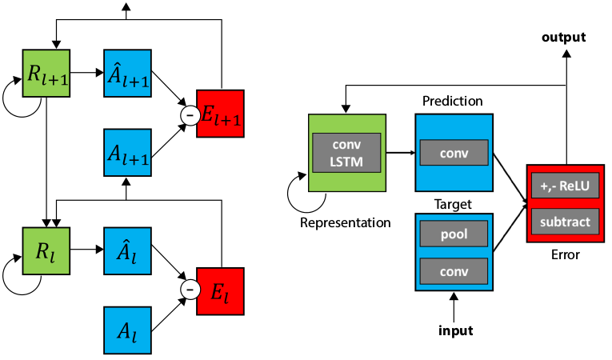
The model learns to maintain a temporally evolving representation of what is going on in the video, because it has recurrent elements. The recurrent elements exist at each depth of the model, so that deeper layers form more abstract and complex representations of the videos. The following figure from the github repository for Prednet describes the basic architecture of the model.
At each depth l, the model has four types of convolutional layers: a recurrent layer (LSTM) R_l, and regular convolutional layers A^hat_l, A_l, and E_l. A represents the input at depth l. This is the current video frame for the most shallow layer of the model. For deeper layers, this is the output of layer E from the previous depth (l - 1). Layer E represents the error in the prediction of the model, that is the difference between A and the prediction of the model Ahat. The prediction Ahat is based on an internal state representation, which is provided by the recurrent layer R.
By passing the error E to next A, deeper layers are required to learn increasingly abstract representations of the task to reduce the overall performance of the model.
Anomaly Detection - Supervised and Unsupervised
Once the model was successfully trained with a dataset that does not contain (m)any anomalies, the model can then be used to detect anomalies. This can be done in a supervised fashion, but you can also perform unsupervised anomaly detection. You can also combine the two approaches, using the output of your neural network for supervised and unsupervised anomaly detection at the same time.
Unsupervised Anomaly Detection
There are several scenarios under which you would perform unsupervised anomaly detection:
- You don't have a labeled dataset. Any supervised approach requires a dataset in which video frames are labeled for whether they contain anomalies.
- You want to be able to detect novel anomalies. If you use a supervised anomaly detection approach, you are limited to detecting anomalies that have occurred in the past.
For these reasons, unsupervised anomaly detection solutions are often preferred. Anomalies are rare (hopefully), so it is often difficult to find a dataset with enough anomalies for training. You also want to be able to detect anomalies that you have never experienced before or that are unique. Imagine an UFO landing on UCSD campus. Would you want be able to detect that UFO the very first time it shows up? Or do you want to rely on an approach where you need to wait until you have enough labeled data to use a supervised approach for UFO detection?
Using unsupervised anomaly detection is as easy as it is versatile. You can simply define a threshold on the model's prediction error for each video frame (e.g. the absolute sum difference between predicted and true pixel values). You then flag all frames as anomalous, for which the error was above that threshold. A slightly more advanced approach would be to deal with possible fluctuations in your data. For example, there are likely more pedestrians on walkways between classes than there are while classes are in session. When there are more pedestrians, the prediction error will overall be higher and you may end up incorrectly flagging a lot of frames as containing anomalies. One options for this scenario would be to send the output of your model to the new Azure cognitive service for anomaly detection.
Supervised Anomaly Detection
The number one reason to use a supervised anomaly detection approach is probably that you could try to categorize anomalies in order to triage tasks to handle them. If your service detects that a crime was committed, it calls campus security or police. If somebody appears to be injured, the service can call an ambulance.
To create a supervised anomaly detection solution, you could train a second model (e.g. a decision tree) on the output of your recurrent model, either features derived from the model's prediction errors or on the activation in one of the hidden layers.
Another approach would be to modify your trained neural network to also have a softmax layer for classifying anomalies in video frames.
Model Development
This is done in the following steps:
- Define the model architecture and optimizer for training it.
- Set up logging so that you can monitor training progress in the Azure portal.
- Connect to your Azure ML workspace.
- Connect to your AML Compute target.
- Define Estimator object.
- Submit your job to your AML experiment for execution.
The first two steps involve changes to a script_file (train.py). The remaining steps are achieved by creating a control script (train_remotely.py) that handles resources and job submission.
Define model Architecture and Optimizer
The first step is to define the model, its inputs and outputs (errors).
# file: train.py
# import custom neural network definition
from prednet import Prednet

# import standard keras modules
import keras
from keras.optimizers import Adam
from keras.layers import Input

# create an instance of the model
prednet = PredNet(output_mode='error')

# define tensor to hold inputs
inputs = Input(n_videoframes, height, width, depth)

# errors will be (batch_size, nt, nb_layers)
errors = prednet(inputs)
The second step is to set up the optimizer for training the model. Here, we are using the Adam optimizer.
# file: train.py
# define optimizer
optimizer = Adam(lr=learning_rate, decay=learning_rate_decay)

# put it all together
model = keras.models.Model(inputs=inputs, outputs=final_errors)
model.compile(loss='mean_absolute_error', optimizer=optimizer)
Above, final_errors is a scalar value derived from errors. See the code repository for details.
Set up logging so that you can monitor training progress in the Azure portal
The next step is to ensure that hyperparameters and training progress are properly logged in your AML workspace so you can monitor performance in the Azure portal while your job is running.
This is how you can log hyperparameters.
# file: train.py
from azureml.core import Run

# log hyper parameters
run.log('learning_rate', learning_rate)
run.log('lr_decay', lr_decay)
To log training progress, we have to create a custom callback for our Keras model.
# file: train.py
from keras.callbacks import Callback

class LogRunMetrics(Callback):
   # callback at the end of every epoch
   def on_epoch_end(self, epoch, log):
      # log a value repeated which creates a list
      run.log('val_loss', log['val_loss'])
      run.log('loss', log['loss'])

callbacks = [LogRunMetrics()]
You can also log an image to your AML workspace. For example, when the training run is complete, you can create a plot with matplotlib to show performance (loss) on the training and the validation set.
# file: train.py

import matplotlib.pyplot as plt
plt.figure(figsize=(6, 3))
plt.title('({} epochs)'.format(nb_epoch), fontsize=14)
plt.plot(history.history['val_loss'], 'b-', label='Validation Loss', lw=4, alpha=0.5)
plt.plot(history.history['loss'], 'g-', label='Train Loss', lw=4, alpha=0.5)
plt.legend(fontsize=12)
plt.grid(True)

run.log_image('Validation Loss', plot=plt)
Set up AML Workspace and Experiment
The AML workspace is awesome for machine learning experimentation.
The workspace is the top-level resource for Azure Machine Learning service. It provides a centralized place to work with all the artifacts you create when you use Azure Machine Learning service.
The workspace keeps a list of compute targets that you can use to train your model. It also keeps a history of the training runs, including logs, metrics, output, and a snapshot of your scripts. You use this information to determine which training run produces the best model.
# file: train_remotely.py
from azureml.core import Workspace, Experiment
ws = Workspace.create(name=workspace_name, subscription_id=azure_subscription_id, resource_group=resource_group, location=azure_region)

exp = Experiment(ws, experiment_name)
For more info on how to setup your AML workspace, go here
Connect to AML Compute target
You can either create a new AML compute target, or connect to an existing one.
The model will be trained on this remote compute target. When you create it, you can specify a couple of important parameters. - vm_size - the size of the compute target. Make sure you pick on with a GPU. Read more here: https://aka.ms/azureml-vm-details. - min_nodes - It's probably best to leave this at the default (0), so that your cluster scales down completely when you don't use it for idle_seconds_before_scaledown (see below), which can save you a lot of money. - max_nodes - Maximum number of nodes to use on the cluster - idle_seconds_before_scaledown - Node idle time in seconds before scaling down the cluster.
# file: train_remotely.py

from azureml.core.compute import AmlCompute
from azureml.core.compute import ComputeTarget

try:
   gpu_compute_target = AmlCompute(workspace=ws, name=gpu_compute_name)
   print("found existing compute target: %s" % gpu_compute_name)
except:
   print('Creating a new compute target...')
   provisioning_config = AmlCompute.provisioning_configuration(vm_size='STANDARD_NC6', max_nodes=5, idle_seconds_before_scaledown=1800)

# create the cluster
gpu_compute_target = ComputeTarget.create(ws, gpu_compute_name, provisioning_config)

# can poll for a minimum number of nodes and for a specific timeout.
# if no min node count is provided it uses the scale settings for the cluster
gpu_compute_target.wait_for_completion(show_output=True, min_node_count=None, timeout_in_minutes=20)
Define Estimator
Estimators are the building block for training. An estimator encapsulates the training code and parameters, the compute resources and runtime environment for a particular training scenario.
# file: train_remotely.py
from azureml.core.container_registry import ContainerRegistry
from azureml.train.estimator import Estimator

# configure access to ACR for pulling our custom docker image
acr = ContainerRegistry()
acr.address = config['acr_address']
acr.username = config['acr_username']
acr.password = config['acr_password']

est = Estimator(source_directory=script_folder,
         compute_target=gpu_compute_target,
         entry_script='train.py',
         use_gpu=True,
         node_count=1,
         custom_docker_image = "wopauli_1.8-gpu:1",
         image_registry_details=acr,
         user_managed=True)
Note how we are using a custom_docker_image. This is because we are using Tensorflow 1.8 and Keras 2.0.8, which are no longer supported by AML services. Apart from that, knowing how to create a custom docker image for training also gives you full control over your execution environment and can speed up provisioning compute targets considerably.
The steps to create a custom docker image are described here.
Submit your job to your AML experiment for execution.
Now we are ready to submit our job to run on our AML compute target. The last line below keeps you connected to the job while it is running remotely, so you can see progress printed on the command line.
# file: train_remotely.py

from azureml.core import Run
run = exp.submit(est)
run.wait_for_completion(show_output=True)
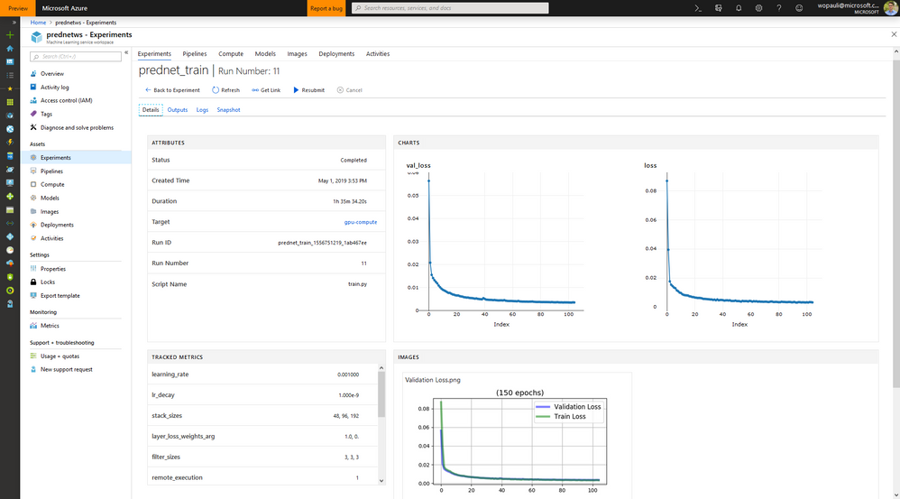
If everything works as expected, you should be able to see progress in the azure portal. Below is what this should look like after a successful training run. You can see Attributes, like how long it ran and what the status is. You can also see Tracked Metrics, which includes hyperparameters and the performance of your model. The performance of the model (training loss and validation loss) are also shown in Charts on the right. Plots like these are automatically created when you log lists of values to the portal.
Download the trained model
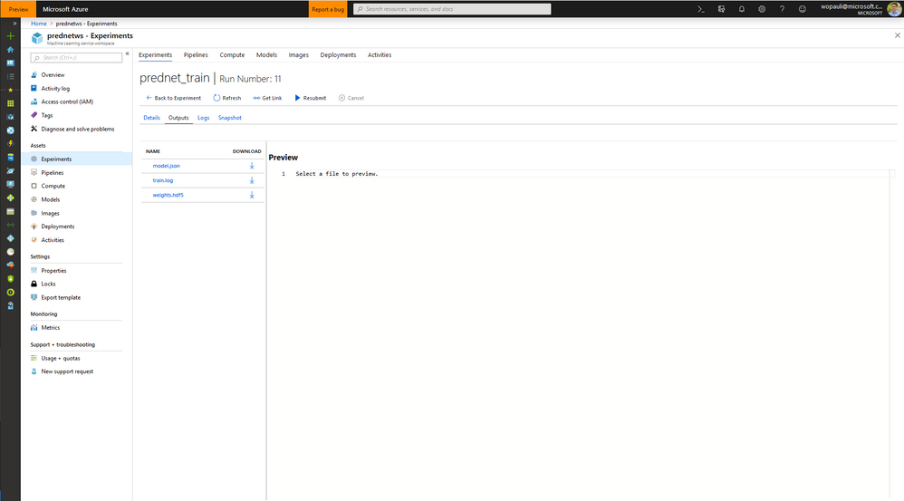
If you go to the panel for Outputs, you can find a your trained model as a json file, with weights saved to a hdf5. To create an anomaly detection solution, you could now download those and run them on your test dataset.
Next steps
Please let me know in the comments below if you found this helpful. Be on the lookout for upcoming blog posts on getting more out of AML services for creating a video anomaly detection service.
Literature
If you want to find out more about anomaly detection, I recommend the following two items.
- Talk at Microsoft Research: Anomaly Detection: Algorithms, Explanations, Applications
- Chandola, V., Banerjee, A., & Kumar, V. (2009). Anomaly detection: A survey. ACM computing surveys (CSUR), 41(3), 15. pdf


