
This post has been republished via RSS; it originally appeared at: Microsoft Research.
In machine learning, adversarial examples usually refer to natural inputs plus small, specially crafted perturbations that can fool the model into making mistakes. In recent years, adversarial examples have been repeatedly discovered in deep learning applications, causing public concerns about AI safety. An illustration of adversarial examples on the image classification task is given below, where an image of a panda is identified as a papillon dog after being altered by small adversarial perturbations, but one should keep in mind that they can cause more destructive problems. For example, adversarial examples have been shown to cause autopilot malfunctions on cars.

Figure 1: an illustration of adversarial perturbations (image by Hadi Salman, Research Engineer at Microsoft)
In a paper titled “Feature Purification: How can Adversarial Training Perform Robust Deep Learning,” researchers from Microsoft Research and Carnegie Mellon University propose the first framework toward understanding the math behind adversarial examples in deep learning. They discovered a principle called “feature purification” that can formally show why a well-trained, well-generalizing ReLU neural network can still be vulnerable to adversarial perturbations on certain datasets and how adversarial training can defend them provably.
Background: Mysteries about adversarial examples and adversarial training
Why do we have adversarial examples? Deep learning models consist of large-scale neural networks with millions of parameters. Due to the inherent complexity of these networks, one school of researchers believe in a “cursed” result: deep learning models tend to fit the data in an overly complicated way so that, for every training or testing example, there exist small perturbations that change the network output drastically. This is illustrated in Figure 2. In contrast, another school of researchers hold that the high complexity of the network is a “blessing”: robustness against small perturbations can only be achieved when high-complexity, non-convex neural networks are used instead of traditional linear models. This is illustrated in Figure 3. It remains unclear whether the high complexity of neural networks is a “curse” or a “blessing” for the purpose of robust machine learning. Nevertheless, both schools agree that adversarial examples are ubiquitous, even for well-trained, well-generalizing neural networks.
 On the other hand, since the discovery of adversarial examples, attempting to design algorithms that find neural networks “robust” to such adversarial examples has been a prevailing research topic. Among the proposed methods, one of the most successful techniques to date is adversarial training, where the algorithm iteratively trains the network with adversarial examples (instead of natural, clean examples) associated with the training set. Nowadays, adversarial training has become a standard empirical tool to improve the neural network robustness. Yet it still remains unclear why, in principle, such adversarial examples exist for well-trained, well-generalizing networks over the original natural dataset and what adversarial training does to networks to defend them against malicious perturbations.
Feature purification: Unraveling the math behind adversarial examples and adversarial training
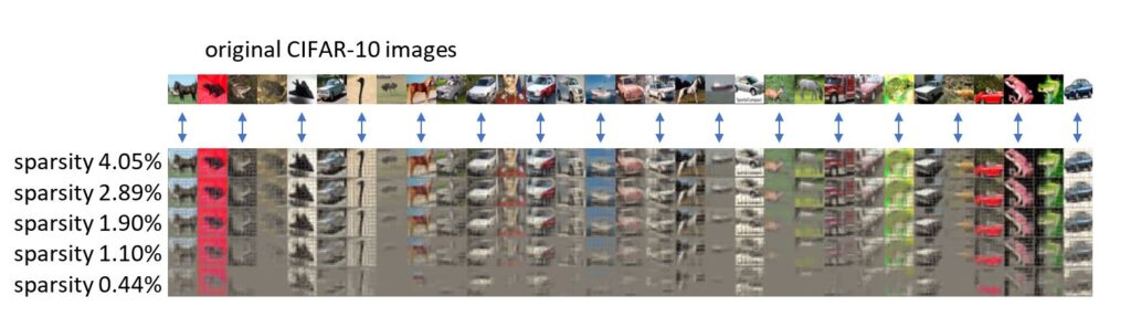
Figure 4: sparse reconstruction of CIFAR-10 images using features from the first layer of AlexNet
The researchers have discovered when the data has a generic structure commonly known as the “sparse coding model,” a model widely used to capture real-world images and texts (see Figure 4). Then, during iterative training, the ReLU network will accumulate, in each neuron, a small “dense mixture direction” that not only has high correlation with the average of their inputs, but also has low correlation with any particular input. Or, in symbols, this can be shown as:

In this equation, d is the dimension, and k/d is the sparsity of the sparse coding model.
The researchers showed that these “dense mixtures” are one of the cruxes of the existence of adversarial examples. These “dense mixtures” have a negligible effect on the original clean data, due to the sparse coding structure, but are extremely vulnerable to adversarial perturbations. Small perturbations along these “dense mixture directions” can alter the network output, for instance from “panda” to “papillon dog” as shown in Figure 1. The researchers also experimentally verified their theory: as shown in the middle row of Figure 5, one can visually verify that the adversarial perturbations are “dense” (that is, they appear like random noise).

Figure 5
Next, the researchers also identified one of the main purposes of adversarial training—to purify those small “dense mixtures” in the features of the network. The principle is summarized as “the principle of feature purification.” To illustrate their theory, Figure 6 plots the visualization of neurons at a certain level in some deep residual network, before and after adversarial training. From this figure one can observe that for individual neurons, their visualization also becomes purified after adversarial training. As another consequence, after adversarial training, one should also expect that the (new) adversarial perturbations will become more “pure,” and this is indeed verified by the last row of Figure 5.

Figure 6: ResNet feature visualization before and after adversarial training
Finally, the researchers also prove that linear models (and several other simple ones), although they can sometimes achieve 100% accuracy on the original dataset, actually lack the power to defend reasonably sized adversarial perturbations. Only high-complexity models, such as ReLU networks, are “blessed” with the capacity to defend against these attacks, but only after adversarial training of course.
To sum up, the researchers have made a first step towards understanding how the features in a neural network are learned during the training process, why after clean training these provably well-generalizing features are still provably non-robust, and why after adversarial training they can be fixed to make the model more robust. The researchers also acknowledge that their finding is still very provisional and have suggested many extensions. For instance, natural images have much richer structures than sparsity; therefore, those “non-robust mixtures” accumulated by clean training might also carry structural properties other than density. Also, they would like to extend their mathematical theorem to capture deeper neural networks, possibly with “hierarchical feature purification” processes, in the spirit of hierarchical learning from their prior work.
The post Newly discovered principle reveals how adversarial training can perform robust deep learning appeared first on Microsoft Research.