This post has been republished via RSS; it originally appeared at: Microsoft Research.
A Generative adversarial network, or GAN, is one of the most powerful machine learning models proposed by Goodfellow et al. for learning to generate samples from complicated real-world distributions. GANs have sparked millions of applications, ranging from generating realistic images or cartoon characters to text-to-image translations. Turing award laureate Yann LeCun called GANs “the most interesting idea in the last 10 years in ML.”
In the context of generating images, GANs consist of two parts. 1) A parameterized (deconvolutional) generator network \(G\) that takes input \(z\) which is a random Gaussian vector and outputs a fake image \(G(z)\). 2) A parameterized (convolutional) discriminator network \(D\) that takes as input an image \(X\)and outputs a real value \(D(X)\). To learn a target distribution \(\mathcal{X}\) of images, the training process of GANs involves finding a generator \(G\) (typically by gradient descent ascent) where the distribution \(G(z)\) of fake images is indistinguishable from the distribution \(\mathcal{X}\) of real images, using any discriminator \(D\) in its parameter family. We illustrate GANs in Figure 1.

GANs are great practically, but what do we know theoretically?
In sharp contrast to the great empirical success, GAN remains one of the least understood machine learning models in theory. How can the generator transfer random vectors from a non-structured spherical Gaussian distribution to highly-structured images? How can the generator be found simply by local search algorithms such as gradient descent ascent (GDA)? What is the role of the discriminator during the training process?
All these theoretical questions remain essentially unanswered. This is perhaps not surprising, since even learning a linear transformation of some known distributions can be computationally hard (even NP-hard in the worst case), not to mention learning a transformation given by neural networks with ReLU activations.
Does it mean GAN theory reaches a dead end? No. To understand the great empirical success of GANs, our new paper “Forward Super-Resolution: How Can GANs Learn Hierarchical Generative Models for Real-World Distributions”, investigates the special structures of real-world distributions, in particular the structure of images, to understand how GANs can work effectively beyond the worst-case, theoretical bounds.
One structural property of real-life images: forward super-resolution
Most real-life images can be viewed in different resolutions without losing the semantics. We often can reduce the resolution of a 1080p car image to as small as, say 16 pixel by 16 pixel, while still maintaining the outline of a car that can be identified by humans.
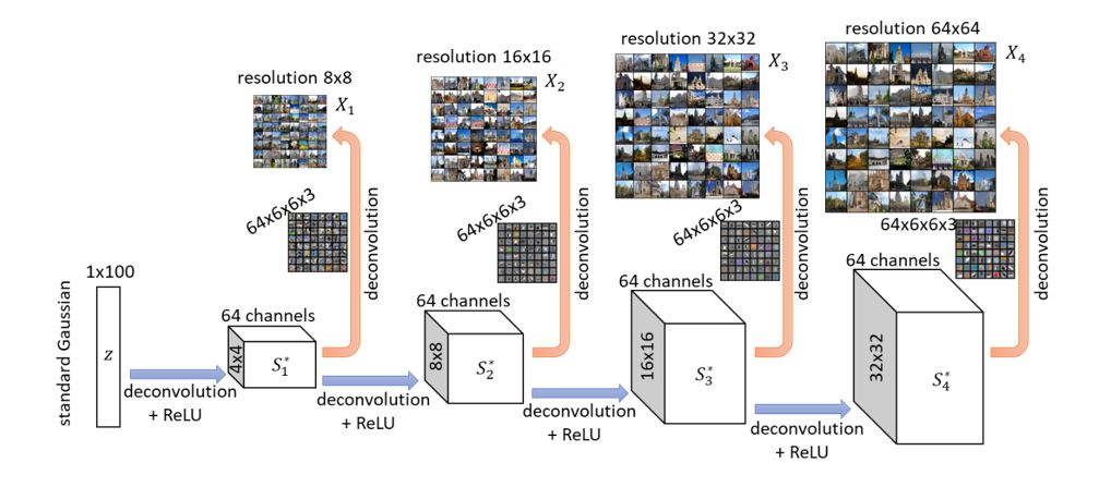
Consequently, one can expect a progressive generative model for real-life images–with the lower layers of the generator producing lower-resolution versions of the images, and higher layers producing higher resolutions. An experimental verification of this progressive generative model was done by NVIDIA researchers Karras et al., and is also illustrated in Figure 2 below.

In this work, we look deeply into this structural property of images. We formalize it as the forward super-resolution property. Mathematically, we consider learning a distribution of images generated progressively as follows. Let \(X_1\),…\(X_{L-1}\) be images of \(X_L\) at lower resolutions (that can be computed from \(X_L\) via image down-scaling), with the resolution of \(X_1\) being the lowest (for example 8×8), and the resolution of \(X_L\) being the highest (for example 128×128). We assume there is a target generator network \(G^*\) (to be learned) with hidden layers \(S{_1^*}\),\(S{_2^*}\),…,\(S{_L^*}\) computed as:
\(S_1\)=\(ReLU(Deconv(z))\), \(S_l\)=\(ReLU(Deconv(\)\(S_{l-1}^*))\)
where \(z\) is a random Gaussian input and Deconv(⋅) is any deconvolution operator (such as nn.ConvTranspose2d in PyTorch). We also assume:
the image \(X_l\) at resolution \(l\) is generated by \(X_l\)=\(Deconv_{output}\)\((S{_l^*})\)
Above, we call \(Deconv_{output}\) (⋅) the output deconvolution layer. They are responsible for representing the “edge-color features” at different resolutions (see Figure 3).

In other words, each hidden layer \(S_l^*\) of the target network \(G\)* is responsible for generating weights to determine “which edge-color features” are to be used to “paint” the output image. The lower-level hidden layers \(S_l^*\) are responsible for generating weights that are used to paint lower-resolution images; and the higher-level hidden layers responsible for painting higher-resolution images.
As a result, when using GANs to learn real-life images, one should expect the higher hidden layers of the learner generator \(G\) to learn – via compositions of hidden deconvolution layers – how to combine lower-resolution features to generate higher-resolution images via super-resolution.
Another structural property of real-life images: hierarchical sparse coding
Real-life images are also very sharp: meaning that one can clearly see the “edge of contrast” at object boundaries and the “consistency of color” within objects in the image. In a generative model, we attribute image sharpness to a hierarchical sparse coding property of hidden layers.
To see this, let us recall that real-life images are usually generated via sparse combinations of “edge-color features” in the output deconvolution layer. For instance (see Figure 4), when a patch in an image is associated with the boundary of an object, an “edge feature” can be selected to generate the pixels in that patch, while all other features become unlikely to show up; in contrast, when a patch is in the middle of an object, a “color feature” can be selected to paint these pixels, while all other features are unlikely to show up.

Mathematically, we model this by assuming for every layer l and every patch p, the restriction of the hidden layer \(S_l^*\) to this patch – denoted by \([S_l^* ]_p\)– is a sparse vector. This means only a few channels are non-zero in every patch (although these non-zero channels can be different at different patches). We have empirically verified this assumption by measuring the sparsity of hidden-layer activations in Figure 5.

How can GANs efficiently learn distributions with forward super-resolution and hierarchical sparse coding?
In this work, we show that the two structural properties of the distributions for images, namely forward super-resolution which ensures semantic consistency of images at different resolutions, and hierarchical sparse coding which ensures image sharpness, are sufficient for GANs to learn such distributions efficiently. Mathematically, we prove the following theorem in our new paper.
Theorem (informal): for any D-dimensional distribution with the forward super-resolution and hierarchical sparse coding properties, for every ε>0, we can learn such distribution up to error ε with sample and time complexity polynomial in D and 1/ε, simply by training GANs using gradient descent ascent (GDA).
In this blog, let us pin down how GANs can learn this distribution without diving into math details. We consider layer-wise training: first train the first layer of the learner generator \(G\) (together with an output deconvolution layer) to generate lowest-resolution images \(X_1\), then train the second layer of \(G\) (together with an output deconvolution layer) to generate \(X_2\), the third layer to generate \(X_3\), and so on. We separate the learning into different phases.
Phase (1). Learn the output deconvolution layers via moment matching
To learn the output deconvolution layers (i.e. the deconvolutional operator from \(X_l\)=\(Deconv_{output}\) \((S_l^* )\) for any layer \(l\)), we show it suffices for the generator to learn to match the moments between the generator’s output images and the target distribution’s real images. This is a special property of distributions generated from the sparse coding model known from earlier theoretical works such as Anandkumar et al.
Intuitively, the output deconvolution layer can be written as a linear operator \(X=Ay\) where each column of matrix A represents an edge-color feature, and y is a sparse vector that determines which edge-color features to use to paint the output image \(X\). It is known under standard regularity conditions (such as almost column orthogonality of \(A\) and sufficient sparsity of \(y\)), for any integer C > 0, the C-th order moment \(\mathbb{E}\)\([X^{⊗C}]≈\) \(∑_i {A_i^{⊗C}} \)\(\mathbb{E}[y{_i^C}]\) where \(A_i\) is the \(i\)-th column of \(A\). When this happens, matching the moments \(\mathbb{E}[X^{⊗C}]\) effectively determines the matrix \(A\) up to a column permutation.
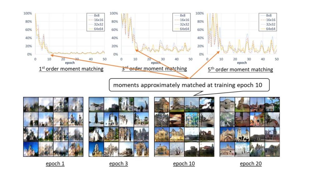
In other words, to learn the output deconvolution layer, it suffices to ensure that the GAN generator matches moments between its output images and real images. On the theoretical side, we show that a ReLU-type discriminator can discriminate the mismatch between the moments on images, and thus through gradient descent ascent the output deconvolution layers can be efficiently learned. On the empirical side, Figure 6 (see also previous work) shows that GANs are indeed doing moment matching during the earlier stage of training.

Phase (2). Learn the first hidden layer via moment matching and sparse decoding
To learn the first hidden layer (i.e. the deconvolutional operator from \((S_{1^*}\)=\(ReLU(Deconv(\)\(z))) \), we show it also suffices to match moments.
Indeed, each coordinate of the first hidden layer \(S{_1^*}\) can be written as \([S{_1^*}]_i\)=\(ReLU(α_i⋅g_i-β_i)\) for \(g_i\) being standard Gaussian. Given the moments of \(S{_1^*}\) even just to any constant order, this uniquely determines \(α_i\) and \(β_i\) for every \(i\) as well as determines the pairwise correlations ⟨\(g_i\), \(g_j\)⟩. In other words, if the discriminator can discriminate the moments of hidden layer \(S_1^*\) from the target generator \(G^*\) and the moments of hidden layer \(S_1\) from the learner generator \(G\), then this effectively determines the first deconvolution layer Deconv(⋅) up to unitary transformation. The main difference from Phase (1) is that, unlike output images, the discriminator does not have access to hidden layer \(S_1^*\) and cannot directly implement this moment matching process.
Fortunately, using the sparse coding property, Phase (1) tells us the discriminator can learn the output deconvolution layers (recall those are “edge-color features”) to descent accuracy, and thus it can use them to perform decoding of \(S_1^*\) from the real images \(X_1\). This requires the first layer of the discriminator to use (approximately) the same set of edge-color features comparing to the output layer of the generator and is consistent to what happens in practice (see Figure 7).

Putting Phases (1) and (2) together, the generator can learn not only the output deconvolution layer but also the first hidden deconvolution layer, and thus learn the distribution of \(X_1\), namely, the “most coarse grind” global structure of the image.
Phase (3). Learn other hidden layers via supervised learning and sparse decoding
For any other hidden layer (i.e. the deconvolutional operator from \(S{_l^*}\)=\(ReLU(Deconv(\)\(S_{l-1}^*))\) for \(l\)≥2), since it captures more and more sharp details of the image, method of moments is no longer known to be sufficient.
In this case, we show the discriminator learns to discriminate the statistical difference of the pair \(((X_{l-1},X_l))\) between real images and \(G\)’s output images. For example, the discriminator can discriminate the case that “a black dot in \(X_2\) always becomes an eye in \(X_3\)” or not. When this is so, the generator can learn how images \(X_{l-1}\) can perform forward super-resolution into \(X_l\), layer by layer for each \(l\)≥2.
The learning process of forward super-resolution should be reminiscent of supervised learning: the goal is to learn a one-hidden-layer neural network that takes as inputs lower-resolution images and outputs higher-resolution ones. Note one main difference from supervised learning is that, in \(S{_l^*}\)=\(ReLU(Deconv(\)\(S_{l-1}^*))\), both the inputs \(S_{l-1}^*\) and the outputs \(S{_l^*}\) are hidden features as opposed to low- and high-resolution images \(X_{l-1}\),\(X_l\). Again, thanks to the sparse coding property and Phase (1), we show that the discriminator can decode these hidden features from their corresponding images \(X_{l-1}\),\(X_l\). This allows GANs to simulate supervised learning and learn how the lower-level features are being combined to generate higher-level features efficiently, purely using gradient descent ascent.

Another key reason that GANs can learn these super-resolution operations efficiently is that such operations are very local: to perform super-resolution on a patch of an image, the generator only needs to look at nearby patches instead of the entire image. Indeed, the global structure has already been taken care of in the lower resolution layers. In other words, learning each hidden layer can be done essentially patch-wise instead of over the entire image, as we illustrate in Figure 9 below.

Empirical evidence of forward super-resolution
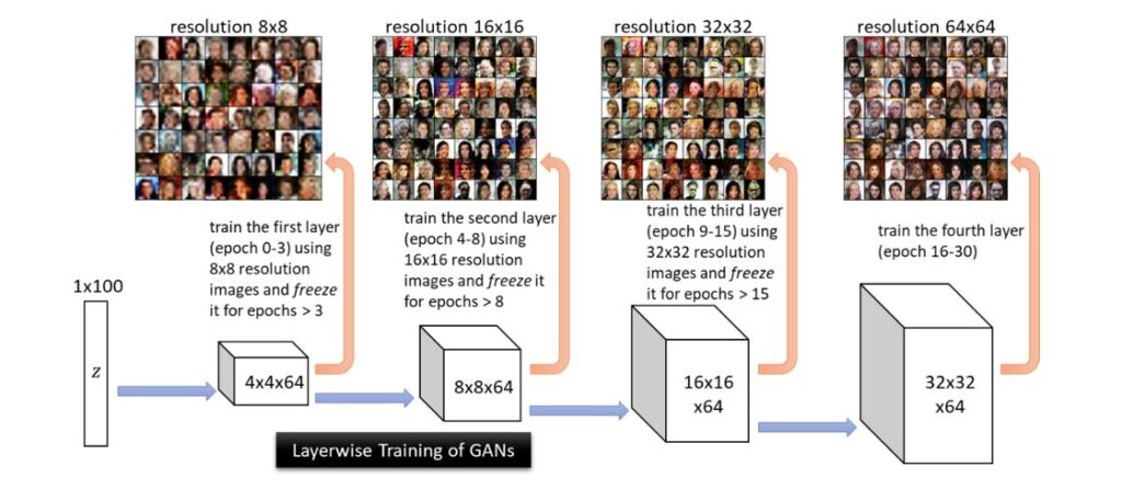
In our work, we also conduct an experiment showing that the features learned from lower-resolution images are indeed extremely helpful for learning higher-resolution images. In Figure 10, we consider layer-wise training of GAN, where we first train only the first hidden layer of the generator, then freeze it and train only the second layer of the generator, and so on. One can obviously see that the features learned from lower-resolution images can indeed be used to generate very non-trivial realistic images at higher resolutions. We believe this is strong evidence that the forward super-resolution property makes the GAN training easy on distributions of real-life images, despite the worst-case hardness bounds.

Next Step: Backward Feature Correction
We point out that our work is still preliminary and far from capturing the full picture of GANs. Most notably, we have focused on the “realizable” setting for proving our main theorem. Thus from a theoretical standpoint, it suffices to perform layer-wise learning: namely, first learn the distribution \(X_1\) and hidden layer \(S_1^*\) , then learn distribution \(X_2\) and hidden layer \(S_2^*\), and so on.
As we show in Figure 10, layer-wise forward super-resolution is already performing much better than learning from random lower-level features. However, in practice we might consider the more challenging “agnostic” setting, where the target distributions of images are generated with error. If we cannot learn hidden layer sufficiently well during layer-wise training, this error propagates to deeper layers and may blow up if we perform layer-wise learning. This is okay for generating simple images, see Figure 10. For more complicated images, we expect the generator network to reduce over-fitting to such errors on lower-level layers, through training higher-level layers altogether. In other words, when training all layers together, we expect the lower-level layers to be able to also capture higher resolution details (as opposed to solely learning lower resolution images). This phenomenon is known as Backward Feature Correction (BFC), which is equipped with provable guarantees in supervised deep learning. Extending the scope of BFC to GANs is an important next step.
The post How can generative adversarial networks learn real-life distributions easily appeared first on Microsoft Research.
