Exploring CPU vs GPU Speed in AI Training: A Demonstration with TensorFlow

This post has been republished via RSS; it originally appeared at: New blog articles in Microsoft Community Hub.

This marks my final blog post of 2023, serving as a fundamental demonstration highlighting the distinctions in speed between CPU and GPU in AI training. The primary aim of this blog is to raise awareness about the accelerated AI training speeds achievable with GPUs. Before delving into the technical details, I'd like to extend my warm wishes for a joyful Christmas and a prosperous New Year in 2024.

In the ever-evolving landscape of artificial intelligence, the speed of model training is a crucial factor that can significantly impact the development and deployment of AI applications. Central Processing Units (CPUs) and Graphics Processing Units (GPUs) are two types of processors commonly used for this purpose. This blog post will delve into a practical demonstration using TensorFlow to showcase the speed differences between CPU and GPU when training a deep learning model.

The main goal of this presentation is to contrast the training speed of a deep learning model on both a CPU and a GPU utilizing TensorFlow. The intention is to offer a lucid comprehension of how the selection of hardware can influence the AI training life cycle, underscoring the importance of GPU acceleration in expediting model training.

Designer (8).jpeg

Before we proceed with the demonstration, let's ensure that the necessary libraries and configurations are in place. We will be using TensorFlow, a popular deep-learning framework. The following Python code snippet checks for the availability of devices in the system and verifies whether TensorFlow is built with CUDA (Compute Unified Device Architecture) support, which is essential for GPU acceleration.

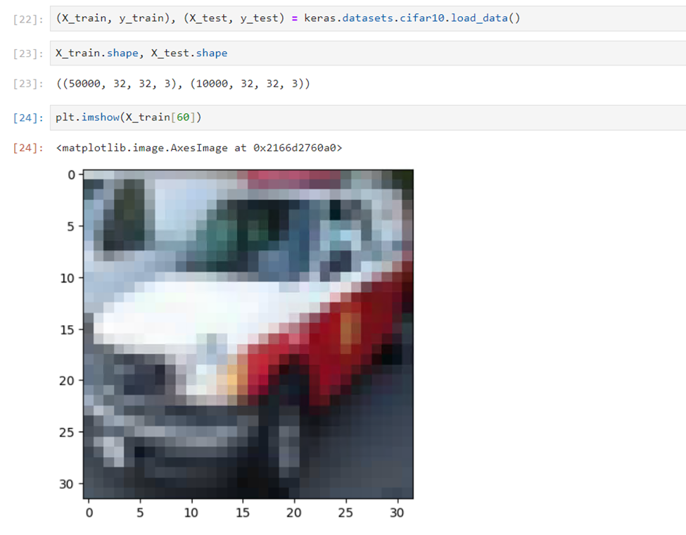
#Importing Libraries import tensorflow as tf from tensorflow import keras import numpy as np import matplotlib.pyplot as plt # Checking available devices tf.config.experimental.list_physical_devices() # Checking if TensorFlow is built with CUDA tf.test.is_built_with_cuda()

For this demonstration, we will use the CIFAR-10 dataset, a well-known dataset in the computer vision community. It consists of 60,000 32x32 color images in 10 different classes. Let's load the dataset, inspect its features, and visualize some images.

#loading the dataset (X_train, y_train), (X_test, y_test) = keras.datasets.cifar10.load_data() # Checking dataset shape and visualizing images X_train.shape, X_test.shape plt.imshow(X_train[60])

To streamline the model training process, it is necessary to scale the images and encode categorical labels. The provided code snippet accomplishes this by scaling the images and transforming the labels into one-hot encoded vectors.

# Scaling the images X_train_scaled = X_train / 255 X_test_scaled = X_test / 255 # Encoding categorical labels y_train_encoded = keras.utils.to_categorical(y_train, num_classes=10, dtype='float32') y_test_encoded = keras.utils.to_categorical(y_test, num_classes=10, dtype='float32')

This code segment normalizes the pixel values of the images by dividing them by 255, effectively scaling them to a range between 0 and 1. Additionally, it utilizes the `to_categorical` function from the Keras library to convert categorical labels into one-hot encoded vectors, facilitating the training of the deep learning model.

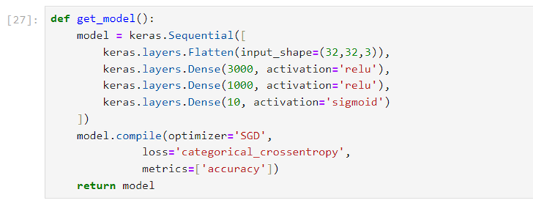
Now, let's define a simple deep-learning model using TensorFlow. The model consists of a flattening layer followed by two dense layers with ReLU activation functions and a final dense layer with a sigmoid activation function.

# Creating the deep learning model def get_model(): model = keras.Sequential([ keras.layers.Flatten(input_shape=(32, 32, 3)), keras.layers.Dense(3000, activation='relu'), keras.layers.Dense(1000, activation='relu'), keras.layers.Dense(10, activation='sigmoid') ]) model.compile(optimizer='SGD', loss='categorical_crossentropy', metrics=['accuracy']) return model

CPU Training Speed

Before proceeding, it's important to note that the provided code is written in a Jupyter Notebook or a similar environment that supports the %%timeit magic command. If you're using a standard Python script or another environment, you may need to adapt the timing measurement accordingly.

Now, let's maintain the structure of your code and provide a clear explanation:

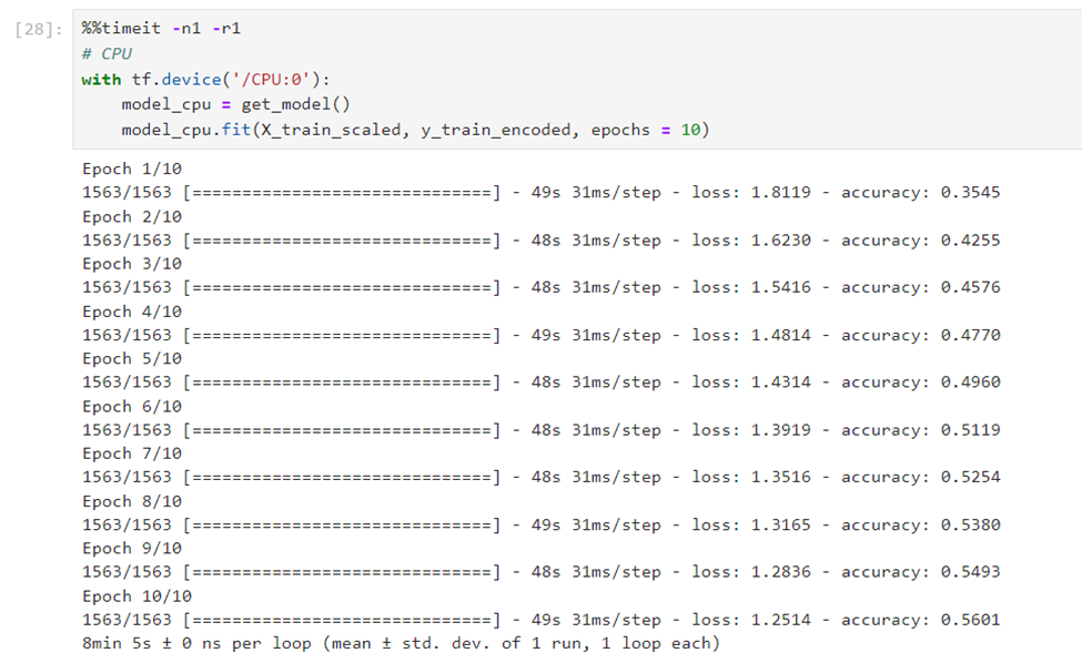
%%timeit -n1 -r1 # Training on CPU with tf.device('/CPU:0'): model_cpu = get_model() model_cpu.fit(X_train_scaled, y_train_encoded, epochs=10)

In this code snippet, the %%timeit magic command is used to measure the execution time of the specified code cell. The options -n1 and -r1 indicate that the cell should be executed once per loop, and the measurement should be repeated only once.

The code itself trains a deep learning model (model_cpu) on the CPU. The get_model() function is assumed to return the architecture of the model. The training data (X_train_scaled and y_train_encoded) is used with the fit method for 10 epochs.

To execute this code in a Jupyter Notebook, you can copy and paste it into a code cell and run the cell. The %%timeit command will provide the average execution time per loop, and the total time taken for the operation will be displayed.

In the obtained results, it's evident that the code required an average of 8 minutes and 5 seconds to finish a single loop of training on the CPU. This duration encompasses both the creation of the model and the training process spanning 10 epochs.

It's important to note that the actual time may fluctuate depending on factors such as the intricacy of your model architecture, the volume of your training data, and the computational capacity of your CPU. These variables play a crucial role in influencing the overall training time and should be considered when assessing performance metrics.

GPU Training Speed

Similar to the CPU example, the %%timeit magic command is used to measure the execution time of the specified code cell. The options -n1 and -r1 indicate that the cell should be executed once per loop, and the measurement should be repeated only once.

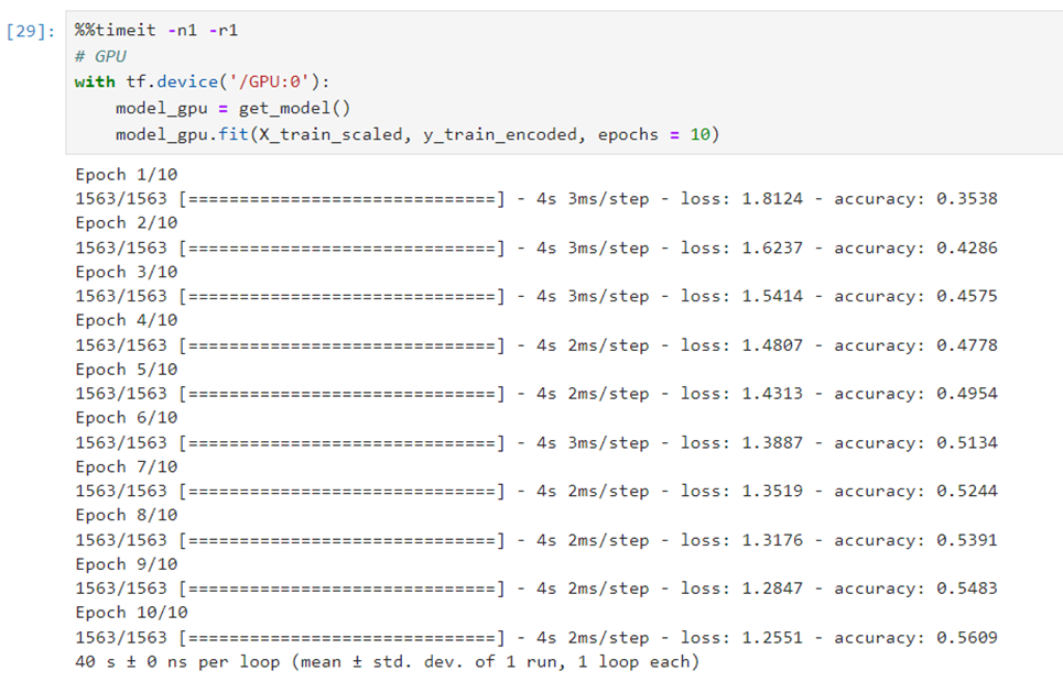
In this code, the with tf.device('/GPU:0') context manager is used to specify that the subsequent operations, including model creation and training, should be executed on the GPU ('/GPU:0'). The get_model() function is assumed to return the architecture of the model. The training data (X_train_scaled and y_train_encoded) is then used with the fit method for 10 epochs.

%%timeit -n1 -r1 # Training on GPU with tf.device('/GPU:0'): model_gpu = get_model() model_gpu.fit(X_train_scaled, y_train_encoded, epochs=10)

The output indicates that the code took an average of 40 seconds to complete one loop of training on the GPU. This measurement includes both the model creation and the training process for 10 epochs.

Comparing this with the CPU training output (8 minutes and 5 seconds), the GPU training is significantly faster, showcasing the accelerated performance that GPUs can provide for deep learning tasks. The reduced time is attributed to the parallel processing capabilities of GPUs, which excel at handling the matrix operations involved in neural network training.

Conclusion:

In conclusion, the demonstration vividly illustrates the substantial difference in training speed between CPU and GPU when utilizing TensorFlow for deep learning tasks. The GPU-accelerated training significantly outperforms CPU-based training, showcasing the importance of leveraging GPU capabilities for expediting the AI model training life cycle. As AI models continue to grow in complexity, the role of GPUs becomes increasingly indispensable, empowering researchers and developers to iterate more efficiently and bring innovative AI solutions to fruition. Choosing the right hardware, such as a GPU, can be a strategic decision in optimizing the overall efficiency and performance of AI applications.

Note: This demonstration is conducted on an Azure Standard NC4as T4 v3 Virtual Machine, equipped with the Nvidia Tesla T4 GPU, utilizing the Microsoft DSVM Image.

Reference:
Microsoft Data Science Virtual Machines
GPU-optimized virtual machine sizes
NCasT4_v3-series

Leave a Reply Cancel reply