
This post has been republished via RSS; it originally appeared at: Microsoft Research.
We are going through a new shift in machine learning (ML), where ML models are increasingly being used to automate decision-making in a multitude of domains: what personalized treatment should be administered to a patient, what discount should be offered to an online customer, and other important decisions that can greatly impact people’s lives.
The machine learning revolution was primarily driven by problems that are distant from such decision-making scenarios. The first scenarios include predicting what an image depicts, predicting the meaning of an English text, or predicting the next frame in a video sequence. This begs the question: is the same hammer used to enable these high-accuracy predictive models equally good enough to drive the nail in automated decision-making? Enter the nascent field of causal machine learning.
Making good decisions requires uncovering causal relationships from data. Causal ML attempts to bridge the gap between prediction and causal inference by utilizing all the recent methodological, technological, and theoretical advances in ML for predictive problems. The field attempts to redirect these advances to address causal problems, many times even using ML out of the box, reducing the causal problem into a sequence of prediction problems that are carefully combined to uncover the causal relationship of interest. You can learn more about this topic and related work across Microsoft Research at the Causality and Machine Learning page.
Our work in “Minimax Estimation of Conditional Moment Models,” accepted at the 34th Conference on Neural Information Processing Systems (NeurIPS2020), and its earlier incarnation in “Adversarial Generalized Method of Moments” is part of this rapidly growing literature in causal ML. In these two works, with fellow Microsoft Research New England researchers Greg Lewis and Lester Mackey along with MIT student Nishanth Dikkala, we propose a novel way of estimating flexible causal models with machine learning from non-experimental data, blending ideas from instrumental variable (IV) estimation from econometrics and generative adversarial networks from machine learning. We’ve made our IV estimation methods open source at our GitHub page.
On the technical level, our work transforms the IV problem into a min-max loss minimization problem—addressable by ML techniques—and develops novel statistical learning theory building on recent work in statistical ML. Before we get into our advances with causal inference and adversarial ML, let’s take a look at why causal inference can lead to ML models that are better suited for decision-making.
Spotlight: Microsoft research newsletter

Microsoft Research Newsletter
Decision-making is about predicting counterfactuals
At its core, the problem with using opaque ML models to enable automated decisions is the discrepancy between correlation and causation. Most ML models achieve high accuracy by taking advantage, in an automated manner, of all correlations that exist in the data to predict what label or outcome is most associated with a given set of features (or variables). Making an optimal decision roughly corresponds to making an intervention and changing one of these features. To make the optimal decision, we need to understand what the outcome would be had we intervened and changed one of the features of a sample. Predicting such counterfactual outcomes requires uncovering the causal relationship between an intervening feature and an outcome, that is understanding the causal effect of that feature on the outcome. Building models of these causal relationships from data is at the core of the overarching field, causal inference.
The problem is that we never observe this counterfactual quantity in the data. Using predictive ML models to essentially “impute” these unobserved quantities runs the risk of relying on correlations in the data that will be broken by interventions and lead to erroneous answers to such “what-if” questions. To make optimal decisions, we need to build causal models that predict counterfactual quantities, in other words what would have happened to the outcome had the decision maker intervened and changed the treatment (also known as action, target feature, driver) to a different, hypothetical value from the one observed in the data.
The big hurdle of causal inference: unobserved confounding
The main hurdle in uncovering causal relationships from non-experimental (observational) data, that is data not coming from an A/B test or a randomized control trial, is unobserved confounding.
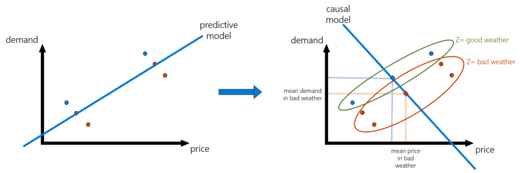
Let’s illustrate this problem with an example. Suppose that we want to set an optimal price for a hotel room, and we have historical data for weekly price and demand (and potentially other observed features associated with each week). It is highly likely that price would increase in historical data in anticipation of high demand due to signals that are only observed by the price setter. For instance, there could be an event happening in town that is not marked in our data, and due to that event, prices for a room surged in that week. At the same time, demand also surged. If we were to train a ML model on such data, we could register this weird correlation that demand increases when price increases and predict that very high prices maximize revenue. This is obviously an erroneous conclusion and portrays the pitfalls of making decisions based on predictive models.

Enter econometrics and instrumental variables. How can we remove biases due to unobserved confounding and get at the causal relationship? Removing such observational biases has been the staple of econometric analysis and more broadly of the field of causal inference. One very popular method used in econometrics is that of instrumental variables, which dates back to very early works in empirical economics in the 1920s (see list of resources at the end of this section).
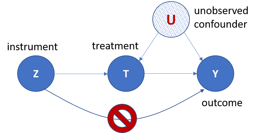
An instrument is an observed variable in the data that affects which action was taken but has no direct causal effect on the outcome of interest. Using another pricing example, suppose that we wanted to identify how demand for coffee in the US is affected by variations in the price. Then we observe that weather in Brazil can affect the production cost of coffee, which can subsequently affect the price of coffee in the US. However, the weather in Brazil has no direct effect on the demand for coffee in the US. Thus, the weather in Brazil can be used as an instrument to uncover the causal relationship between price and demand in the US. Though the process of identifying a valid instrument is a delicate task, as it is context-specific and requires domain knowledge, using instrumental variables is a ubiquitous approach in causal inference.
Angrist, J. D., & Pischke, J.-S. (2008). Mostly Harmless Econometrics: An Empiricist’s Companion. Princeton university press.
Imbens, G. W., & Rubin, D. B. (2015). Causal Inference for Statistics, Social, and Biomedical Sciences: An Introduction. Cambridge University Press. doi:10.1017/CBO9781139025751
Pearl, J. (2009). Causality. Cambridge University Press.
Wright, P. G. (1928). Tariff on Animal and Vegetable Oils. Macmillan Company, New York.
Instrumental variables (IV) with machine learning
However, most estimation approaches that use instrumental variables make heavy assumptions on the causal model. For instance, the most widespread method, called two-stage-least-squares (2SLS), requires that the relationship between the treatment and the outcome be linear. Such linearities are oftentimes violated in real-world scenarios: demand typically does not vary linearly with price and all other observable features typically do not enter linearly in this relationship.
To make causal estimation more robust, we need to be able to estimate more flexible causal models. ML has exactly succeeded in this topic: fitting flexible models from data, in a data-adaptive manner, without suffering from the curse of dimensionality—the fact that most classical non-parametric methods in statistics require an unreasonably large number of samples even with a very modest number of features.
Motivating questions: Empowering non-parametric instrumental variable methods with machine learning
Can we use all the recent algorithmic advances in supervised ML (such as deep neural networks, high-dimensional penalized linear models, kernel regression, and random forests) to fit causal models when we have access to an instrument? Moreover, can we use recent advances in statistical ML to prove more robust statistical estimation theorems for non-parametric instrumental variable estimation methods that adapt to the intrinsic dimensionality and complexity of the true causal model?
The non-parametric instrumental variable problem has a long history in econometrics and tackles exactly the problem of estimating flexible causal models with instruments (see resource list at end of section). However, in addition to existing methods typically suffering from the curse of dimensionality, many times their guarantees require strong assumptions on the data-generating process. Our work builds on this marvelous econometric theory and attempts to merge it with techniques from ML to make non-parametric IV have a more widespread applicability.
The discrepancy. The merging of the two worlds is not obvious. Supervised ML is traditionally formulated as minimizing an expected loss under a test population (a model formalized by the statistical learning theory framework).
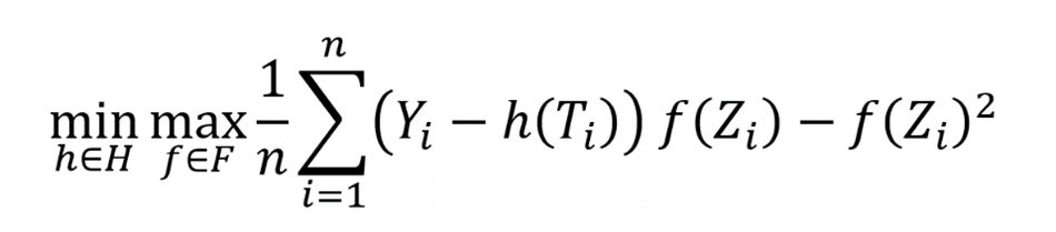
It’s not clear which loss function can best emulate the solution to the instrumental variable problem. The starting point of causal model identification and estimation with instruments is a conditional moment assumption that the data-generating process needs to satisfy. Namely, we assume that the variation in the outcome \(Y\) that cannot be causally explained by the treatment \(T\) (formally the quantity \(Y\)–\(h(T)\), where \(h\) is the causal model) is not predictable at all from the instrument \(Z\) (going back to our coffee pricing example, roughly speaking unobserved events in the US that vary the demand are not predictable by weather in Brazil). More formally, we assume that for any value of the instrument \(Z\):
\(E[Y -h(T)∣ Z]= 0 \)How do we turn such a conditional moment assumption into a loss to optimize? The main idea of our work is that we can frame the solution to the latter infinite set of conditions (one for every value of Z), as an adversarial learning problem, the solution to a zero-sum game.
Blundell, R., Chen, X., & Kristensen, D. (2007). Semi-nonparametric IV estimation of shape-invariant Engel curves. Econometrica, 75, 1613–1669.
Chen, X., & Christensen, T. M. (2018). Optimal sup-norm rates and uniform inference on nonlinear functionals of nonparametric IV regression. Quantitative Economics, 9, 39–84.
Chen, X., & Pouzo, D. (2012).
Estimation of nonparametric conditional moment models with possibly nonsmooth generalized residuals. Econometrica, 80, 277–321.
Darolles, S., Fan, Y., Florens, J.-P., & Renault, E. (2011). Nonparametric instrumental regression. Econometrica, 79, 1541–1565.
Hall, P., & Horowitz, J. L. (2005). Nonparametric methods for inference in the presence of instrumental variables. The Annals of Statistics, 33, 2904–2929.
Horowitz, J. L. (2011).
Applied nonparametric instrumental variables estimation. Econometrica, 79, 347–394.
Newey, W. K., & Powell, J. L. (2003). Instrumental variable estimation of nonparametric models. Econometrica, 71, 1565–1578.
Causal inference meets adversarial learning
Adversarial learning is a relatively novel technique in ML and has been very successful in training complex generative models with deep neural networks based on generative adversarial networks, or GANs. In GANs, a generative model of the data is trained by viewing the problem as a zero-sum game having one player (generator) generate artificial samples based on some deep neural network representation of the probability distribution of the data and an adversary (discriminator) that tries to distinguish between the artificial and real samples.
If a generator succeeds in fooling the discriminator, then it must have learned an accurate description of the data-generating process. In the adversarial formulation of the instrumental variable problem (more generally, statistical problems defined via conditional moment constraints), the analog of the generator is trying to generate a good causal model \(h\), while the analog of the discriminator is trying to find a combination of the moment constraints that are violated.
We can phrase this more technically as finding the solution to the following min-max problem:
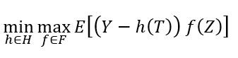
where \(H\) is a hypothesis/function space that we believe our causal model lies in (for example, a neural net, a random forest, a high-dimensional linear function, a reproducing kernel Hilbert space) and \(F\) is some flexible test function space. Thus, we have turned the IV problem into a loss minimization problem, hopefully addressable by many ML algorithms and such that we can analyze it with modern machinery from statistical ML.
Technical advances: Statistical learning theory for min-max losses
The min-max nature of the loss presents many technical difficulties both in terms of practical implementations and in terms of theoretical analysis. Most recent algorithms and statistical advances in ML deal with smooth convex losses in the model’s output, while the “max” in the objective function creates inherent non-smoothness. Moreover, convexity is very brittle as the zero-sum game’s loss is linear in the model’s output. Our work proposes that this discrepancy can be alleviated by adding a strongly convex penalty term to the minimax formulation:
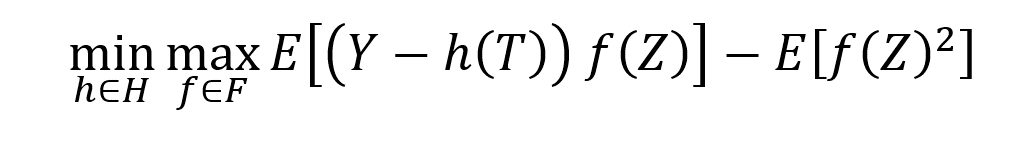
This modification intuitively penalizes moment constraints that have high variance and technically offers the desired strong-convexity and smoothness to the objective.
Statistics. Given this modification, we can analyze the estimation rate of causal models that are the result of solving an empirical analogue of the above loss function, when given access to \(n\) datapoints:
We show that as long as the function space \(F\) is rich enough (formally, it contains differences between any two functions in \(H\) projected on the instrument, represented in the equation \(E\)\([h(T)\)–\(h’\)\((T)│Z]\)) then the machinery of localized Rademacher analysis, introduced in the last two decades in statistical learning theory, governs the estimation rate of such min-max estimates. The resulting error bound is many times statistically minimax optimal. The existing localized Rademacher theory has been applied to smooth losses that do not possess such a complicated min-max structure. Thus, one can view our theoretical advancement as an extension of this machinery to adversarial learning problems.
Algorithmics. On the computational side, we show how to solve the empirical min-max problem for many function spaces of interest. For instance, we propose computationally efficient algorithms for penalized linear models, for reproducing kernel Hilbert spaces, for spaces defined via shape constraints, and for random forests. We also offer heuristic methods for the case of neural networks, inspired by the algorithmic approaches proposed for training GANs. Finally, we show that generically, under mild assumptions, one can computationally reduce the min-max problem at hand, to a regression and a classification oracle. This ultimately enables all algorithmic techniques developed for these basic ML problems to be applicable to the IV problem.
How our work moves causal inference forward
There has been a surge of methods providing more flexible approaches to causal estimation with instruments, using ML techniques, either prior to our work (DeepIV) and following the earlier incarnation of our work (DeepGMM, DualIV, KernelIV, KernelMMR). Some highlights that differentiate our contribution:
- Prior works focus on a particular ML approach, such as neural networks or reproducing kernel Hilbert spaces.
- Prior works do not offer tight estimation rates that are enabled by our localized Rademacher analysis of min-max problems.
- No prior work has enabled estimation of the non-parametric IV problem with random forests or with shape constraints.
We cannot possibly do justice to these works within the space constraints of this blog post, and we defer the reader to the extended related work in our paper for a more detailed comparison. Moving forward, we view the use of adversarial ML as a tool that can empower several econometric and causal inference techniques beyond the instrumental variable setting that we outline in this work.
All our IV estimation methods are available as open source at our GitHub page.
The post Adversarial machine learning and instrumental variables for flexible causal modeling appeared first on Microsoft Research.