This post has been republished via RSS; it originally appeared at: Excel Blog articles.
| Round 1 Post | Round 2 Post | Round 3 Post |
Link to Test 3 Workbook - WITHOUT answers
Link to Test 3 Workbook - WITH answers
Finally, the round 3 post is here! Since my last post, we held the world finals round,
named our Canada Champ
This post warrants the warning: my videos are still long. I get started talking about Excel and can’t stop! Because the video explanations are long, I’m going to try keeping this write up short. If the post doesn’t give you enough info, check the video. When the video is not good enough, hit the web and USE THE COMMUNITY! That’s why we are all here.
Challenge 01-01 (Data Relays part 1)
The purpose of this question was to get deeper into Get & Transform, which I LOVE. Get & Transform (aka PowerQuery) and the Data Model together is an insanely powerful combination. It dramatically changed the way I did my job when I was as a financial analyst. Building up skills on both tools can be a huge time saver when it comes to analytical work, and they are shared technologies between Excel and PowerBI
The other thing I will say (repeat of a comment in the video) is that there are many ways to get the answer. I’ve taken a path that intentionally uses lots of queries to show you the capability of modularizing your queries to use them as building blocks for one another (a great way to avoid repeating work and a way to make updates automatically flow through all your query work) Okay, onto to the nitty gritty.
- Get Data From Race 1 (2:22) – we'll figure out all the shaping for Race 1, then repeat the steps for 2 and 3.
- [Race 1] Create a new Athlete Birthday Column (2:52) – we will need this to calculate ages
- [Race 1] Create a new Age column (4:52) – Age equals Race Date minus Birthday (we divide the number of days by 365 to get years). There are a variety of DateTime/Duration functions in the M query language you could leverage. I took this approach to mirror how you might calculate the age in a traditional Excel spreadsheet
- [Race 1] Sort athletes by result time (7:00) – so we can calculate athlete ranks in the race (who came in 1st, 2nd, 3rd, etc…)
- [Race 1] Add an Race Rank column (7:35) – we can determine ranks with the table sorted by adding an index column
- [Race 2] Repeat steps 1-5 for Race 2 (10:00)
- [Race 3] Repeat steps 1-5 for Race 3 (11:35)
- Combine all the Race Data (13:40) – Get & Transform makes this easy with the append queries capability
- Find all the 1st place and 2nd place Race Winners (17:00) – this was the first way athletes could qualify for the finals. We just need a quick filtering of the race ranks. We'll put these names in a separate query to access later
- Find the other 2 qualifying finalists (22:00) – this was the second way athletes could qualify for the finals. We do this by filtering out the 1st/2nd place winners, and then do the same sort/index column approach we did in step 5. The top 2 "remaining" athletes are the other finalists. We'll put these names in a separate query to access later. Note: I intentionally took a separate step here to show you how conditionals (if formulas) work in queries. If you have questions about setup or syntax, check out the end of this step.
- Combine the 2 queries that identify Finalists (28:30) – append queries, sort as required (result time and athlete number), and delete columns we do not need.
Challenge 01-02 (Data Relays part 2)
TIME FOR THE DATA MODEL! The data model allows you to work with massive amounts of data (millions of rows), easily connect different data sets together via relationships, and run complex, dynamic calculations. Now, this is an introduction. We are just trying to get folks comfortable with the data model, before we unleash its awesome power! I HIGHLY recommend using some of the community resources/trainings for the data model. It really is a game changing technology for spreadsheet analytics. Again, the steps below are short and to the point. The video gives some deeper explanations of the data model for all the newbies out there. If you just want the answers, read below. If you want to get the details (and can bear listening to me) watch the video.
- Get Data Tables into the Data Model (1:45) – we use get and transform to get the data and check the “Add this data to the Data Model” rather than having the query results output to a table on a worksheet.
- Build a relationship between the tables (9:00) – it’s an easy drag and drop to make a relationship, but this means our data tables are connected and the data model understands how a column in one table matches a country in another table. Before the data model, you probably built relationships by taking one data table and pulling in columns from a second table by doing a VLOOKUP based off a column with matching values between the 2 tables.
- Create an average result time measure (17:30) – we now use DAX formula language to build this measure. We’ll be using a simple function, AVERAGE. Spreadsheet pros should be familiar with this one
- Sort the countries in the pivot by result times (25:25)
Challenge 02 (Chart Gymnastics)
Just like my prior posts, I won’t go into a lot of details here. There is no right answer. If you are new to chart building, go check out some of the references I provided in the round 1 post.
We selected this data set to see how people would handle separate but related data. The challenge asked comeptitors to
- compare individual event scores
- compare total scores
- show how event
Showing all this at once is a tough thing to do. Naturally the community rose to the challenge!
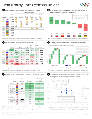
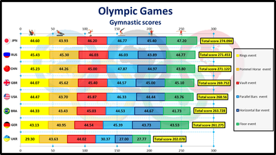
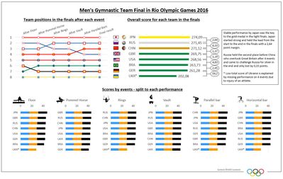
Take a look at some of our most popular visualizations from this round….
| link to post | link to post | link to post |
 |
 Espero les guste y suerte para todos, han llegado hasta aquí, siéntanse orgullosos Espero les guste y suerte para todos, han llegado hasta aquí, siéntanse orgullosos |
 |
Challenge 03 (Formula Wrestling)
Questions 1-3 are pretty straightforward because we thought questions 4 and 5 would be complex. So I won’t say a lot here in the write up. Check the video. Questions 1-3 are short and sweet answers.
Questions 4 and 5 have some extra comments in the file to help explain what’s going on. Again, use the video for questions 4 and 5. I mentioned in the video that the most formula “efficient” submissions for questions 4 and 5 used a brut force technique of calculating all possible routes in the map. This never crossed our minds as an option when we wrote the challenge. Well done outsmarting us! That said I wanted show some of the interesting ways you can leverage Excel formulas, so my answer implements Dijkstra's algorithm. For those of you not familiar Dijkstra’s algorithm, it is an approach to navigating nodes with connecting paths with of varying weights. The nodes and paths could represent traffic travel times, the speed of telecommunications transmissions, the costs of airline routes, etc… Check out this Wikipedia article on Dijkstra’s algorithm as a reference for the video.
Also, I start the video by saying I made it short and sweet. That ended up being a lie – sorry. I started talking, and you know how that goes…
- How many sections of roads are closed? (2:29) – we use COUNTIF to count the closed roads (count cells equal to 999)
- What percent of “open” sections of roads are busy? (3:00) – we need a fraction.
- The numerator equals the count of busy sections.
We use COUNTIFS to specify busy roads as those with travel time greater than 10 minutes but not closed). - The denominator equals the count of open sections of roads
We just COUNT all sections of road and subtract the closed sections (the answer to question 1)
- The numerator equals the count of busy sections.
- What is the average travel time (in minutes) on “clear” sections of road? (4:50) – AVERAGEIF makes it easy to find just the clear sections of road (travel time less than or equal to 10 minutes) for our calculation.
- What is the fastest possible travel time (in minutes) from Venue A to Venue F (5:55) – As I said, the video gets into a thorough explanation of the solution. I hope between the video and the comments in the file you should be able to track what all is going on. The formula concepts are not new, we leverage MIN/MAX, INDEX, MATCH, IF, and string concatenation. All of which we used in prior rounds. The one explanation will add here is the OFFSET formula. The online documentation for OFFSET is great. I’ll give the short version here…
OFFSET lets you point at 1 cell, then shift up or down a certain number of rows, shift left or right a certain number of columns, and return that new cell. For example OFFSET(A1, 2, 1) returns cell B3 because A1 shifted 2 rows is A3 then shifted 1 column is B3. You can do that shift over and then return a block of cells by using the optional height/width parameters of the formula.
By making your row/column shift numbers formulas, you can do dynamic offsets. In this solution, I use MATCH to look up a value among column/row labels of a matrix. Tucking these MATCH caclulations inside my OFFSET formula, I traverse the matrix and extract values…to find the travel time from venue E to venue B, start at the upper left corner of the travel times table, shift down until you are in the “E” row, then shift right until you are in the “B” column - See Question 4 (watch the video)
There you have it, I know it’s a short write-up, but this is really a case where the video serves you much better than words. I loved trying to figure out how to implement Dijkstra’s algorithm. Hopefully you enjoyed the challenges and the solutions here.
More posts on the remaining tests will be coming (I swear) and thanks in advance for your patience.
As always, thanks for visiting the community!
| Round 1 Post | Round 2 Post | Round 3 Post |
